| SOCR ≫ | DSPA ≫ | Topics ≫ |
Data Science and Predictive Analytics (UMich HS650)
Deep Learning, Neural Networks
SOCR/MIDAS (Ivo Dinov)
July 2017
Deep learning is a special branch of machine learning using a collage of algorithms to model high-level motifs in data. Deep learning resembles the biological communications between brain neurons in the central nervous system (CNS), where synthetic graphs represent the CNS network as pairs of nodes and connections/edges between them. For instance, in a simple synthetic network consisting of a pair of connected nodes, an output send by one node is received by the other as an input signal. When more nodes are present in the network, they may be arranged in multiple levels (like a multiscale object) where the \(i^{th}\) layer output serves as the input of the next \((i+1)^{st}\) layer. The signal is manipulated at each layer and sent as a layer output downstream and interpreted as an input to the next, \((i+1)^{st}\) layer, and so forth. Deep learning relies on many layers of nodes, many edges linking the nodes, forming input/output (I/O) layered grids representing a multiscale processing network. At each layer, linear and non-linear transformations are converting inputs into outputs.
In this chapter, we explore the R deep learning package MXNetR and demonstrate state-of-the-art deep learning models utilizing CPU and GPU for fast training (learning) and testing (validation). Other powerful deep learning frameworks include TensorFlow, Theano, Caffe, Torch, CNTK and Keras.
Neural Networks vs. Deep Learning: Deep Learning is a machine learning strategy that learns a deep multi-level hierarchical representation of the affinities and motifs in the dataset. Machine learning Neural Nets tend to use shallower network models. Although there are no formal restrictions on the depth of the layers in a Neural Net, few layers are commonly utilized. Recent methodological, algorithmic, computational, infrastructure and service advances overcome previous limitations. In addition, the rise of Big Data accelerated the evolution of classical Neural Nets to Deep Neural Nets, which can now handle lots of layers and many hidden nodes per layer. The former is a precursor to the latter, however, there are also non-neural deep learning techniques. For example, syntactic pattern recognition methods and grammar induction discover hierarchies.
1 Deep Learning Training
Review Chapter 10 (Black Box Machine-Learning Methods: Neural Networks and Support Vector Machines) prior to proceeding.
1.1 Perceptrons
A perceptron is an artificial analogue of a neuronal brain cell that calculates a weighted sum of the input values and outputs a thresholded version of that result. For a bivariate perceptron, \(P\), having two inputs, \((X,Y)\), denote the weights of the inputs by \(A\) and \(B\), respectively. Then, the weighted sum could be represented as: \[W = A X + B Y.\]
At each layer \(l\), the weight matrix, \(W^{(l)}\), has the following properties:
- The number of rows of \(W^{(l)}\) equals the number of nodes/units in the previous \((l-1)^{st}\) layer, and
- The number of columns of \(W^{(l)}\) equals the number of units in the next \((l+1)^{st}\) layer.
Neuronal cells fire depending on the presynaptic inputs to the cell which causes constant fluctuations of the neuronal the membrane - depolarizing or hyperpolarizing, i.e., the cell membrane potential rises or falls. Similarly, perceptrons rely on thresholding of the weight-averaged input signal, which for biological cells corresponds to voltage increases passing a critical threshold. Perceptrons output non-zero values only when the weighted sum exceeds a certain threshold \(C\). In terms of its input vector, \((X,Y)\), we can describe the output of each perceptron (\(P\)) by:
\[ Output(P) = \left\{ \begin{array} {} 1, & if A X + B Y > C \\ 0, & if A X + B Y \leq C \end{array} \right. \]
Feed-forward networks are constructed as layers of perceptrons where the first layer ingests the inputs and the last layer generates the network outputs. The intermediate (internal) layers are not directly connected to the external world, and are called hidden layers. In fully connected networks, each perceptron in one layer is connected to every perceptron on the next layer enabling information “fed forward” from one layer to the next. There are no connection between perceptrons in the same layer.
Multilayer perceptrons (fully-connected feed-forward neural network) consist of several fully-connected layers representing an input matrix \(X_{n \times m}\) and a generated output matrix \(Y_{n \times k}\). The input \(X_{n,m}\) is a matrix encoding the \(n\) cases and \(m\) features per case. The weight matrix \(W_{m,k}^{(l)}\) for layer \(l\) has rows (\(i\)) corresponding to the weights leading from all the units \(i\) in the previous layer to all of the units \(j\) in the current layer. The product matrix \(X\times W\) has dimensions \(n\times k\).
The hidden size parameter \(k\), the weight matrix \(W_{m \times k}\), and the bias vector \(b_{n \times 1}\) are used to compute the outputs at each layer:
\[Y_{n \times k}^{(l)} =f_k^{(l)}\left ( X_{n \times m} W_{m \times k}+b_{k \times 1} \right ).\]
The role of the bias parameter is similar to the intercept term in linear regression and helps improve the accuracy of prediction by shifting the decision boundary along \(Y\) axis. The outputs are fully-connected layers that feed into an activation layer to perform element-wise operations. Examples of activation functions that transform real numbers to probability-like values include,
- the sigmoid function, a special case of the logistic function, which converts real numbers to probabilities,
- the rectifier (
relu, Rectified Linear Unit) function, which outputs the \(\max(0, input)\), - the tanh (hyperbolic tangent function).

The final fully-connected layer may be hidden of size equal to the number of classes in the dataset and may be followed by a softmax layer mapping the input into a probability score. For example, if a size \({n\times m}\) input is denoted by \(X_{n\times m}\), then the probability scores may be obtained by the softmax transformation function, which maps real valued vectors to vectors of probabilities:
\[\left ( \frac{e^{x_{i,1}}}{\displaystyle\sum_{j=1}^m e^{x_{i,j}}},\ldots, \frac{e^{x_{i,m}}}{\displaystyle\sum_{j=1}^m e^{x_{i,j}}}\right ).\]
Below is a schematic of fully-connected feed-forward neural network of nodes \[ \{ a_{j=node\ index, l=layer\ index} \}_{j=1, l=1}^{n_j, 4}.\]

The plot above illustrates the key elements in the action potential, or activation function, calculations and the corresponding training parameters: \[a_{node=k,layer=l} = f\left ( \displaystyle\sum_{i}{w_{k,i}^l \times a_{i}^{l-1} +b_{k}^l} \right ),\] where:
- \(f\) is the activation function, e.g., logistic functin \(f(x) = \frac{1}{1+e^{-x}}\). It converts the aggregate weights at each node to probability values,
- \(w_{k,i}^l\) is the weight carried from the \(i^{th}\) element of the \((l-1)^{th}\) layer to the \(k^{th}\) element of the current \(l^{th}\) layer,
- \(b_{k}^l\) is the (residual) bias present in the \(k^{th}\) element in the \(l^{th}\) layer. This is effectively the information not explained by the training model.
These parameters may be estimated using different techniques (e.g., using least squares, or stochastically using steepest decent methods) based on the training data.
2 Biological Relevance
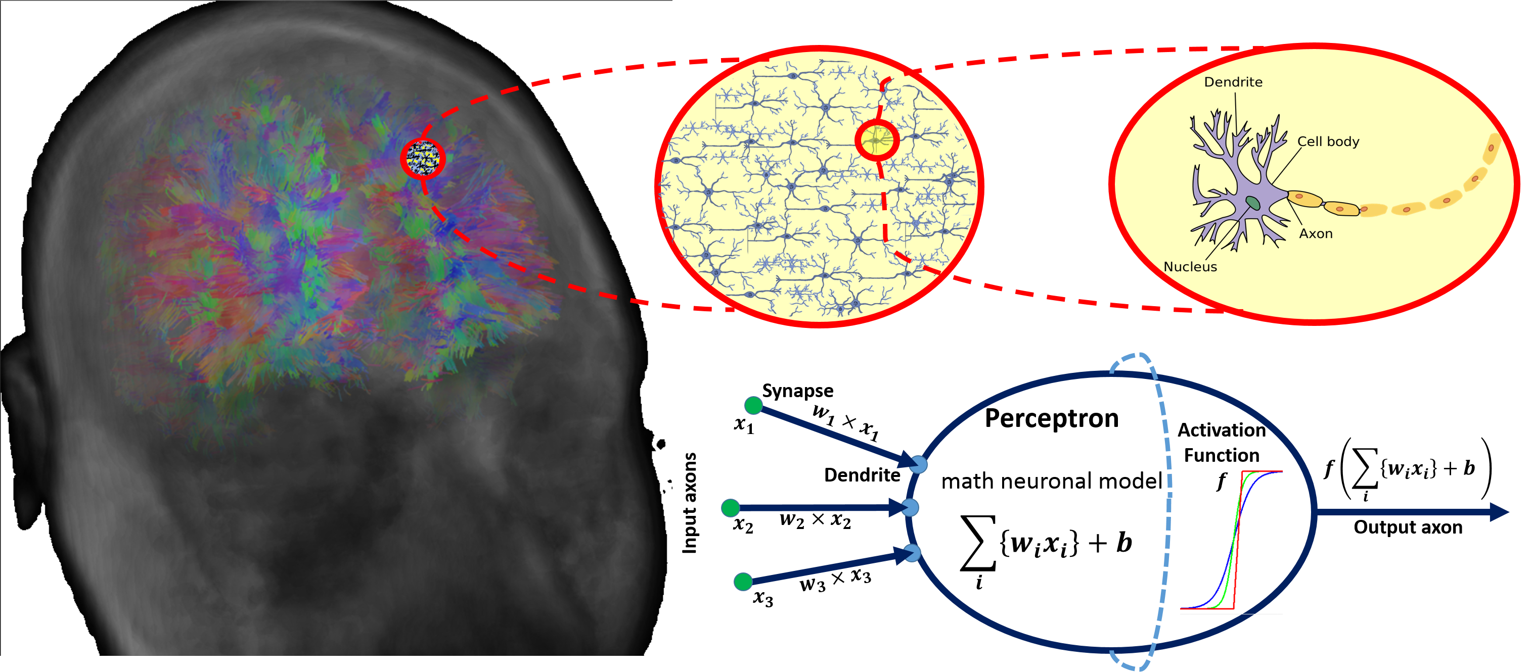
There are parallels between biology (neuronal cells) and the mathematical models (perceptrons) for neural network representation. The human brain contain about \(10^{11}\) neuronal cells connected by approximately \(10^{15}\) synapses forming the basis of our functional phenotypes. The schematic below illustrates some of the parallels between brain biology and the mathematical representation using synthetic neural nets. Every neuronal cell receives multi-channel (afferent) input from its dendrites, generates output signals and disseminates the results via its (efferent) axonal connections and synaptic connections to dendrites of other neurons.
The perceptron is a mathematical model of a neuronal cell that allows us to explicitly determine algorithmic and computational protocols transforming input signals into output actions. For instance, signal arriving through axon \(x_0\) is modulated by some prior weight, e.g., synaptic strength, \(w_0\times x_0\). Internally, within the neuronal cell, this input is aggregated (summed, or weight-averaged) with inputs from all other axons. Brain plasticity suggests that synaptic strengths (weight coefficients \(w\)) are strengthened by training and prior experience. This learning process controls the direction and strength of influence of neurons on other neurons. Either excitatory (\(w>0\)) or inhibitory (\(w\leq 0\)) influences are possible. Dendrites and axons carry signals to and from neurons, where the aggregate responses are computed and transmitted downstream. Neuronal cells only fire if action potentials exceed a certain threshold. In this situation, a signal is transmitted downstream through its axons. The neuron remains silent, if the summed signal is below the critical threshold.
Timing of events is important in biological networks. In the computational perceptron model, a first order approximation may ignore the timing of neuronal firing (spike events) and only focus on the frequency of the firing. The firing rate of a neuron with an activation function \(f\) represents the frequency of the spikes along the axon. We saw some examples of activations functions earlier.
The diagram below illustrates the parallels between the brain network-synaptic organization and an artificial synthetic neural network.
3 Simple Neural Net Examples
Before we look at some examples of deep learning algorithms applied to model observed natural phenomena, we will develop a couple of simple networks for computing fundamental Boolean operations.
3.1 Exclusive OR (XOR) Operator
The exclusive OR (XOR) operator works as a bivariate binary-outcome function, mapping pairs of false (0) and true (1) values to dichotomous false (0) and true (1) outcomes.
We can design a simple two-layer neural network that calculates XOR. The values within each neurons represent its explicit threshold, which can be normalized so that all neurons utilize the same threshold, typically \(1\)). The value labels associated with network connections (edges) represent the weights of the inputs. When the threshold is not reached, output is \(0\), and then the threshold is reached, the output is correspondingly \(1\).

Let’s work out manually the 4 possibilities:
| InputX | InputY | XOR Output(Z) |
|---|---|---|
| 0 | 0 | 0 |
| 0 | 1 | 1 |
| 1 | 0 | 1 |
| 1 | 1 | 0 |
We can validate that this network indeed represents an XOR operator by plugging in all four possible input combinations and confirming the expected results at the end.

3.2 NAND Operator
Another binary operator is NAND (negative AND, Sheffer stroke) that produces a false (0) output if and only if both of its operands are true (1), and generates true (1), otherwise. Below is the NAND input-output table.
| InputX | InputY | XOR Output(Z) |
|---|---|---|
| 0 | 0 | 1 |
| 0 | 1 | 1 |
| 1 | 0 | 1 |
| 1 | 1 | 0 |
Similarly to the XOR operator, we can design a one-layer neural network that calculates NAND. The values within each neurons represent its explicit threshold, which can be normalized so that all neurons utilize the same threshold, typically \(1\)). The value labels associated with network connections (edges) represent the weights of the inputs. When the threshold is not reached, the output is trivial (\(0\)) and when the threshold is reached, the output is correspondingly \(1\). Here is a shorthand analytic expression for the NAND calculation:
\[NAND(X,Y) = 1.3 - (1\times X + 1\times Y).\] Check that \(NAND(X,Y)=0\) if and only if \(X=1\) and \(Y=1\), otherwise it equals \(1\).

3.3 Complex networks designed using simple building blocks
Observe that stringing some of these primitive networks together, or/and increasing the number of hidden layers, allows us to model problems with exponentially increasing complexity. For instance, constructing a 4-input NAND function would simply require repeating several of our 2-input NAND operators. This will increase the space of possible outcomes from \(2^2\) to \(2^4\). Of course, introducing more depth in the hidden layers further expands the complexity of the problems that can be modeled using neural nets.
You can interactively manipulate the Google’s TensorFlow Deep Neural Network Webapp to gain additional intuition and experience with the various components of deep learning networks.
The ConvnetJS demo provide another hands-on example using 2D classification with 2-layer neural network.
4 Classification
In MXNet, Multilayer perceptron (MLP) may be defined by:
- Creating a place holder variable for the input data,
data = mx.sym.Variable('data') - Flattening the data from 4D shape space (width, height, batch_size, num_channel) into 2D (num_channel*width*height, batch_size), ’data = mx.sym.Flatten(data=data)`
- And iterating over the fully-connected layers:
- First layer,
fc1 = mx.sym.FullyConnected(data=data, name='fc1', num_hidden=128) - Apply
relufunction to the output of the first fully-connnected layer,act1 = mx.sym.Activation(data=fc1, name='relu1', act_type="relu") - Generate the second fully-connected layer and apply the activation function,
fc2 = mx.sym.FullyConnected(data=act1, name='fc2', num_hidden = 64); act2 = mx.sym.Activation(data=fc2, name='relu2', act_type="relu") Generate the third/final fully-connected layer, with a hidden size \(k=10\), which in digit recognition tasks corresponds to the number of unique digits \(0:9]\),
fc3 = mx.sym.FullyConnected(data=act2, name='fc3', num_hidden=10)Finally, mapping the input into a probability score using the softmax and loss layer,
mlp = mx.sym.SoftmaxOutput(data=fc3, name='softmax'). See the mlp R source code here.
4.1 Sonar data example
Let’s load the mlbench and mlbench packages and demonstrate the basic invocation of mxnet. The Sonar data mlbench::Sonar includes sonar signals bouncing off a metal cylinder or a roughly cylindrical rock. Each of 208 patterns includes a set of 60 numbers (features) in the range 0.0 to 1.0, and a label (M or R). Each feature represents the energy within a particular frequency band, integrated over a certain period of time. The M and R labels associated with each record rock or mine (metal cylinder). The numbers in the labels are in increasing order of aspect angle, but they do not encode the angle directly.
# Load the required packages: mlbench and mxnet
# install.packages("mlbench"); install.packages("mxnet")
# Note mxnet requires "visNetwork"
# If it doesn't work, you may need the following lines:
# install.packages("drat", repos="https://cran.rstudio.com")
# drat:::addRepo("dmlc")
# install.packages("mxnet")
require(mlbench)
require(mxnet)## Init Rcppdata(Sonar, package="mlbench")
table(Sonar[,61])##
## M R
## 111 97Sonar[,61] = as.numeric(Sonar[,61])-1 # R = "1", "M" = "0"
set.seed(123)
train.ind = sample(1:nrow(Sonar),0.7*nrow(Sonar))
train.x = data.matrix(Sonar[train.ind, 1:60])
train.y = Sonar[train.ind, 61]
test.x = data.matrix(Sonar[-train.ind, 1:60])
test.y = Sonar[-train.ind, 61]Let’s start by using a multi-layer perceptron as a classifier. The mxnet function mx.mlp builds a general multi-layer neural network that can be utilized to do classification or regression graph modeling. It relies on the following parameters:
- Training data and labels
- Number of hidden nodes in each hidden layers
- Number of nodes in the output layer
- Type of activation
- Type of output loss
- The device to train (GPU or CPU)
- Additional optional parameters, see
mx.model.FeedForward.create
Here is one example using the training and testing data we defined above:
mx.set.seed(1234)
model.mx <- mx.mlp(train.x, train.y, hidden_node=8, out_node=2, out_activation="softmax",
num.round=200, array.batch.size=15, learning.rate=0.1, momentum=0.9,
eval.metric=mx.metric.accuracy,verbose=F)
#calculate Prediction sensitivity & specificity
preds = predict(model.mx, test.x) # these are probabilities
# You can inspect the test labels vs. assigned probabilities by
# View(data.frame(test.y, preds[2,]))
preds1 <- ifelse(preds[2,] <= 0.5, 0, 1) # dichotomize to labels
table(preds1)## preds1
## 0 1
## 35 28pred.label = t(preds1)
table(pred.label, test.y)## test.y
## pred.label 0 1
## 0 28 7
## 1 6 22library("caret")## Loading required package: lattice## Loading required package: ggplot2sensitivity(factor(preds1), factor(as.numeric(test.y)),positive = 1)## [1] 0.7586207specificity(factor(preds1), factor(as.numeric(test.y)),negative = 0)## [1] 0.8235294We can also use crossval::diagnosticErrors() and crossval::confusionMatrix() to get more detailed evaluations. Similar to sensitivity() and specificity(), we should specify the negative and positive labels.
Note that you have to specify crossval::confusionMatrix() if you also have the caret package loaded, as caret also has a function called confusionMatrix().
library("crossval")##
## Attaching package: 'crossval'## The following object is masked from 'package:caret':
##
## confusionMatrixdiagnosticErrors(crossval::confusionMatrix(preds1,test.y, negative = 0))## acc sens spec ppv npv lor
## 0.7936508 0.7857143 0.8000000 0.7586207 0.8235294 2.6855773
## attr(,"negative")
## [1] 0Now, we compare the results of different number of rounds.
mx.set.seed(1234)
get_pred = function(n){
model.mx <- mx.mlp(train.x, train.y, hidden_node=8, out_node=2, out_activation="softmax",
num.round=n, array.batch.size=15, learning.rate=0.1, momentum=0.9,
eval.metric=mx.metric.accuracy,verbose=F)
preds = predict(model.mx, test.x)
}
preds100 = get_pred(100)
preds50 = get_pred(50)
preds10 = get_pred(10)We can plot the ROC curve and calculate the AUC (Area under the curve):
# install.packages("pROC"); install.packages("plotROC"); install.packages("reshape2")
library(pROC); library(plotROC); library(reshape2); ## Type 'citation("pROC")' for a citation.##
## Attaching package: 'pROC'## The following objects are masked from 'package:stats':
##
## cov, smooth, var# compute AUC
get_roc = function(preds){
roc_obj <- roc(test.y, preds[2,])
auc(roc_obj)
}
get_roc(preds)## Area under the curve: 0.9249get_roc(preds100)## Area under the curve: 0.9209get_roc(preds50)## Area under the curve: 0.8824get_roc(preds10)## Area under the curve: 0.8022#plot roc
dt <- data.frame(test.y, preds[2,], preds100[2,], preds50[2,], preds10[2,])
colnames(dt) <- c("D","rounds=200","rounds=100","rounds=50","rounds=10")
dt <- melt(dt,id.vars = "D")
basicplot <- ggplot(dt, aes(d = D, m = value, colour=variable)) + geom_roc(labels = FALSE, size = 0.5, alpha.line = 0.6, linejoin = "mitre") +
theme_bw() + coord_fixed(ratio = 1) + style_roc() + ggtitle("ROC CURVE")+
annotate("rect", xmin = 0.4, xmax = 1, ymin = 0.2, ymax = 0.75,
alpha = .2)+
annotate("text", x = 0.7, y = 0.5, size = 3,
label = "AUC: \n rounds=200: 0.9209\n rounds=100: 0.9128\n rounds=50: 0.8824\n rounds=10: 0.8022\n " )
basicplot
The plot suggests that the results stabilize after 100 iterations.
Let’s look at some visualizations of the real labels of the test data (test.y) and their corresponding ML-derived classification labels (preds[2,]) using 200 iterations.
graph.viz(model.mx$symbol)hist(preds10[2,],main = "rounds=10")
hist(preds50[2,],main = "rounds=50")
hist(preds100[2,],main = "rounds=100")
hist(preds[2,],main = "rounds=200")
We see a significant bimodal trend when the number of rounds increases. Another plot may be generated by:
library(ggplot2)
get_gghist = function(preds){
ggplot(data.frame(test.y, preds),
aes(x=preds, group=test.y, fill=as.factor(test.y)))+
geom_histogram(position="dodge",binwidth=0.25)+theme_bw()
}
df = data.frame(preds[2,],preds100[2,],preds50[2,],preds10[2,])
p <- lapply(df,get_gghist)
require(gridExtra) # used for arrange ggplots## Loading required package: gridExtragrid.arrange(p$preds10.2...,p$preds50.2...,p$preds100.2...,p$preds.2...)
4.2 MXNet Notes
The
mx.mlp()function is a proxy to the more complex and laborious process of defining a neural network by using MXNet’sSymbol. For instance, this callmodel.mx <- mx.mlp(train.x, train.y, hidden_node=8, out_node=2, out_activation="softmax", num.round=20, array.batch.size=15, learning.rate=0.1, momentum=0.9, eval.metric=mx.metric.accuracy)would be equivalent to a symbolic network definition like:data <- mx.symbol.Variable("data"); fc1 <- mx.symbol.FullyConnected(data, num_hidden=128) act1 <- mx.symbol.Activation(fc1, name="relu1", act_type="relu"); fc2 <- mx.symbol.FullyConnected(act1, name="fc2", num_hidden=64); act2 <- mx.symbol.Activation(fc2, name="relu2", act_type="relu"); fc3 <- mx.symbol.FullyConnected(act2, name="fc3", num_hidden=2); lro <- mx.symbol.SoftmaxOutput(fc3, name="sm"); model2 <- mx.model.FeedForward.create(lro, X=train.x, y=train.y, ctx=mx.cpu(), num.round=100, array.batch.size=15, learning.rate=0.07, momentum=0.9)(see example with linear regression below).- Layer-by-layer definitions translate inputs into outputs. At each level, the network allows for a different number of neurons and alternative activation functions. Other options can be specified by using
mx.symbol: mx.symbol.Convolutionapplies convolution to the input and then adds a bias. It can create convolutional neural networks.mx.symbol.Deconvolutiondoes the opposite and can be used in segmentation networks along withmx.symbol.UpSampling, e.g., to reconstruct the pixel-wise classification of an image.mx.symbol.Poolingreduces the data by selecting signals with the highest response.mx.symbol.Flattenlinks convolutional and pooling layers to form a fully connected network.mx.symbol.Dropoutattempts to cope with the overfitting problem.
The function mx.mlp() is a wrapper for quick design of standard multi-layer perceptrons. For more extensive experiments, customized symbolic representation can be explicitly specified using combinations of the above methods.
# Example of **LeNet** network for recognizing handwritten digits:
data <- mx.symbol.Variable('data')
conv1 <- mx.symbol.Convolution(data=data, kernel=c(5,5), num_filter=20)
tanh1 <- mx.symbol.Activation(data=conv1, act_type="tanh")
pool1 <- mx.symbol.Pooling(data=tanh1, pool_type="max", kernel=c(2,2), stride=c(2,2))
conv2 <- mx.symbol.Convolution(data=pool1, kernel=c(5,5), num_filter=50)
tanh2 <- mx.symbol.Activation(data=conv2, act_type="tanh")
pool2 <- mx.symbol.Pooling(data=tanh2, pool_type="max", kernel=c(2,2), stride=c(2,2))
flatten <- mx.symbol.Flatten(data=pool2)
fc1 <- mx.symbol.FullyConnected(data=flatten, num_hidden=500)
tanh3 <- mx.symbol.Activation(data=fc1, act_type="tanh")
fc2 <- mx.symbol.FullyConnected(data=tanh3, num_hidden=10)
lenet <- mx.symbol.SoftmaxOutput(data=fc2)
model <- mx.model.FeedForward.create(lenet, X=train.x, y=train.y, ctx=device.cpu, num.round=5, array.batch.size=100, learning.rate=0.05, momentum=0.9)To allow smooth, fast, and consistent operation on CPU and GPU, in in mxnet, the generic R function controlling the reproducibility of stochastic results is overwritten by mx.set.seed. So can use mx.set.seed() to control random numbers in MXNet.
To examine the accuracy of the model.mx learner (trained on the training data), we can make prediction (on testing data) and evaluate the results using the provided testing labels (report the confusion matrix).
preds = predict(model.mx, test.x)
pred.label = max.col(t(preds))-1
table(pred.label, test.y)## test.y
## pred.label 0 1
## 0 28 7
## 1 6 22For multi-class predictions, mxnet outputs \(n\ (class) \times m\ (examples)\) confusion matrices where each row corresponds to probability of the corresponding (column-defined) class.
5 Case-Studies
Let’s demonstrate regression and prediction deep learning examples using several complementary datasets.
5.1 ALS regression example
Let’s first demonstrate a deep learning regression using the ALS data to predict ALSFRS_slope.
als <- read.csv("https://umich.instructure.com/files/1789624/download?download_frd=1")
als <- scale(als[,-c(1,7)])
train.ind = sample(1:nrow(als),0.7*nrow(als))
train.x = data.matrix(als[train.ind,-c(1,7)])
train.y = als[train.ind,7]
test.x = data.matrix(scale(als[-train.ind,-c(1,7)]))
test.y = als[-train.ind,7]
# Define the input data
data <- mx.symbol.Variable("data")
# A fully connected hidden layer
# data: input source
# num_hidden: number of neurons in this hidden layer
fc1 <- mx.symbol.FullyConnected(data, num_hidden=1)
# Use linear regression for the output layer
lro <- mx.symbol.LinearRegressionOutput(fc1)
mx.set.seed(1234)
# Create a MXNet Feedforward neural net model with the specified training.
model <- mx.model.FeedForward.create(lro, X=train.x, y=train.y,
ctx=mx.cpu(), num.round=1000, array.batch.size=20,
learning.rate=2e-6, momentum=0.9, eval.metric=mx.metric.rmse,verbose = F)## Warning in mx.model.select.layout.train(X, y): Auto detect layout of input matrix, use rowmajor..The option verbose = F can suppress messages including training accuracy report in each iteration. You may rerun the code with verbose = T to examine the rate of decrease of train error against the number of iterations.
You must scale data before input it into MXnet, which expects that the training and testing sets are normalized to the same scale. There are two strategies to scale the data.
- Either scaling the complete data simultaneously and then split them into train data and test data, or
- Scale only the training data set to enable model-training, but save your protocol for data normalization, as new data (testing, validation) will need to be (pre)processed the same way as the training data.
Have a look at the Google TensorFlow API. It shows the importance of learning rate and the number of rounds. You should test different sets of parameters.
- Too small learning rate may lead to long computations.
- Too large learning rate may cause the algorithm to fail to converge, as large step size (learning rate) may by-pass the optimal solution and then oscillate or even diverge.
preds = predict(model, test.x)## Warning in mx.model.select.layout.predict(X, model): Auto detect layout of input matrix, use rowmajor..sqrt(mean((preds-test.y)^2))## [1] 0.2171032range(test.y)## [1] -3.181499 1.943890We can see that the RMSE on the test set is pretty small. To get a visual representation of the deep learning network we can also display this relatively simple computation graph:
graph.viz(model$symbol)5.2 Spirals 2D Data
We can again use the mx.mlp wrapper to construct the learning network, but we can also use a more flexible way to construct and configure the multi-layer network in mxnet. This configuration is done by using the Symbol call, which specifies the links among network nodes, the activation function, dropout ratio, and so on:
Below we show configuration of perceptron with one hidden layer.
########### Network configuration
# variables
act <- mx.symbol.Variable("data")
# affine transformation
fc <- mx.symbol.FullyConnected(act, num.hidden = 10)
# non-linear activation
act <- mx.symbol.Activation(data = fc, act_type = "relu")
# affine transformation
fc <- mx.symbol.FullyConnected(act, num.hidden = 2)
# softmax output and cross-
mlp <- mx.symbol.SoftmaxOutput(fc)
####Preparing data
set.seed(2235)
############ spirals dataset
s <- sample(x = c("train", "test"), size = 1000, prob = c(.8,.2), replace = TRUE)
dta <- mlbench.spirals(n = 1000, cycles = 1.2, sd = .03)
dta <- cbind(dta[["x"]], as.integer(dta[["classes"]]) - 1)
colnames(dta) <- c("x","y","label")
######### train, validate, test
dta.train <- dta[s == "train",]
dta.test <- dta[s == "test",]Let’s display the data and examine its structure.
dt <- as.data.frame(dta);dt[,3] <- as.factor(dt[,3])
dt.train <- dt[s == "train",]
dt.test <- dt[s == "test",]
p1 <- ggplot(dt,aes(x = x,y = y,color=label))+geom_point()+ggtitle("Whole data structure")
p2 <- ggplot(dt.train,aes(x = x,y = y,color=label))+geom_point()+ggtitle("Train data structure")
p3 <- ggplot(dt.test,aes(x = x,y = y,color=label))+geom_point()+ggtitle("Test data structure")
grid.arrange(p1,p2,p3,nrow=3)
# Network training
# Feed-forward networks may be trained using iterative gradient descent algorithms. A **batch** is a subset of data that is used during single forward pass of the algorithm. An **epoch** represents one step of the iterative process that is repeated until all training examples are used.
############ basic spiral-data training
mx.set.seed(2235)
model <- mx.model.FeedForward.create(
symbol = mlp,
X = dta.train[, c("x", "y")],
y = dta.train[, c("label")],
num.round = 500,
array.layout = "rowmajor",
learning.rate = 1,
eval.metric = mx.metric.accuracy,verbose = F)
preds = predict(model, dta.test[,c(1:2)])## Warning in mx.model.select.layout.predict(X, model): Auto detect layout of input matrix, use rowmajor..pred.label = max.col(t(preds))-1; table(pred.label, dta.test[,3])##
## pred.label 0 1
## 0 90 30
## 1 22 73The prediction result is close to perfect and we can inspect deeper the results using crossval::confusionMatrix.
library("crossval")
diagnosticErrors(crossval::confusionMatrix(pred.label,dta.test[,3],negative = 0))## acc sens spec ppv npv lor
## 0.7581395 0.7684211 0.7500000 0.7087379 0.8035714 2.2980293
## attr(,"negative")
## [1] 0ggplot(data.frame(dta.test[,3], preds[2,]),
aes(x=preds[2,], group=dta.test[,3], fill=as.factor(dta.test[,3])))+
geom_histogram(position="dodge",binwidth=0.25)+theme_bw()
Once we fit a model (like the binary label classification below), we can:
- Visually inspect the quality of the ML classification.
- Display the structure of the labeled test-data objects.
# define a custom call-back, which stops the process of training when the progress in accuracy is below certain level of tolerance. It call is made after every epoch to check the status of convergence of the algorithm.
mx.callback.train.stop <- function(tol = 1e-3, mean.n = 1e2, period = 100, min.iter = 100) {
function(iteration, nbatch, env, verbose = TRUE) {
if (nbatch == 0 & !is.null(env$metric)) {
continue <- TRUE
acc.train <- env$metric$get(env$train.metric)$value
if (is.null(env$acc.log)) {
env$acc.log <- acc.train
} else {
if ((abs(acc.train - mean(tail(env$acc.log, mean.n))) < tol &
abs(acc.train - max(env$acc.log)) < tol &
iteration > min.iter) |
acc.train == 1) {
cat("Training finished with final accuracy: ",
round(acc.train * 100, 2), " %\n", sep = "")
continue <- FALSE
}
env$acc.log <- c(env$acc.log, acc.train)
}
}
if (iteration %% period == 0) {
cat("[", iteration,"]"," training accuracy: ",
round(acc.train * 100, 2), " %\n", sep = "")
}
return(continue)
}
}
###### training with custom stopping
mx.set.seed(2235)
model <- mx.model.FeedForward.create(
symbol = mlp,
X = dta.train[, c("x", "y")],
y = dta.train[, c("label")],
num.round = 2000,
array.layout = "rowmajor",
learning.rate = 1,
epoch.end.callback = mx.callback.train.stop(),
eval.metric = mx.metric.accuracy,
verbose = FALSE
) ## [100] training accuracy: 75.56 %
## [200] training accuracy: 76 %
## [300] training accuracy: 76 %
## [400] training accuracy: 76.45 %
## Training finished with final accuracy: 76.45 %labeled_spiral_data <- as.data.frame(cbind(dta.test[, c("x", "y")], as.factor(pred.label)))
colnames(labeled_spiral_data) <- c("x", "y", "label")
labeled_spiral_data$label <- as.factor(labeled_spiral_data$label)
p4 <- ggplot(labeled_spiral_data, aes(x = x,y = y,color=label))+geom_point()+ggtitle("Structure of Predicted-Labels on Test Data")
p4
5.3 IBS Study
Let’s try another example using the IBS NI Study data.
# IBS NI Data
# UCLA Data
wiki_url <- read_html("http://wiki.stat.ucla.edu/socr/index.php/SOCR_Data_April2011_NI_IBS_Pain")
IBSData<- html_table(html_nodes(wiki_url, "table")[[2]]) # table 2
set.seed(1234)
test.ind = sample(1:354, 50, replace = F) # select 50/354 of cases for testing, train on remaining (354-50)/354 cases
# UMich Data (includes MISSING data): use `mice` to impute missing data with mean: newData <- mice(data,m=5,maxit=50,meth='pmm',seed=500); summary(newData)
# wiki_url <- read_html("http://wiki.socr.umich.edu/index.php/SOCR_Data_April2011_NI_IBS_Pain")
# IBSData<- html_table(html_nodes(wiki_url, "table")[[1]]) # load Table 1
# set.seed(1234)
# test.ind = sample(1:337, 50, replace = F) # select 50/337 of cases for testing, train on remaining (337-50)/337 cases
# summary(IBSData); IBSData[IBSData=="."] <- NA; newData <- mice(IBSData,m=5,maxit=50,meth='pmm',seed=500); summary(newData)
html_nodes(wiki_url, "#content")## {xml_nodeset (1)}
## [1] <div id="content">\n\t\t<a name="top" id="top"></a>\n\t\t\t\t<h1 id= ...# View (IBSData); dim(IBSData): Select an outcome response "DX"(3), "FS_IQ" (5)
# scale/normalize all input variables
IBSData <- na.omit(IBSData)
IBSData[,4:66] <- scale(IBSData[,4:66]) # scale the entire dataset
train.x = data.matrix(IBSData[-test.ind, c(4:66)]) # exclude outcome
train.y = IBSData[-test.ind, 3]-1
test.x = data.matrix(IBSData[test.ind, c(4:66)])
test.y = IBSData[test.ind, 3]-1
# View(data.frame(train.x, train.y))
# View(data.frame(test.x, test.y))
# table(test.y); table(train.y)
# num.round - number of iterations to train the model
act <- mx.symbol.Variable("data")
fc <- mx.symbol.FullyConnected(act, num.hidden = 10)
act <- mx.symbol.Activation(data = fc, act_type = "sigmoid")
fc <- mx.symbol.FullyConnected(act, num.hidden = 2)
mlp <- mx.symbol.SoftmaxOutput(fc)
mx.set.seed(2235)
model <- mx.model.FeedForward.create(
symbol = mlp,
array.batch.size=20,
X = train.x, y=train.y,
num.round = 200,
array.layout = "rowmajor",
learning.rate = exp(-1),
eval.metric = mx.metric.accuracy, verbose=FALSE)
preds = predict(model, test.x)
pred.label = max.col(t(preds))-1; table(pred.label, test.y)## test.y
## pred.label 0 1
## 0 23 10
## 1 10 7library("crossval")
diagnosticErrors(crossval::confusionMatrix(pred.label,test.y,negative = 0))## acc sens spec ppv npv lor
## 0.6000000 0.4117647 0.6969697 0.4117647 0.6969697 0.4762342
## attr(,"negative")
## [1] 0ggplot(data.frame(test.y, preds[2,]),
aes(x=preds[2,], group=test.y, fill=as.factor(test.y)))+
geom_histogram(position="dodge",binwidth=0.25)+theme_bw()
# convert pred-probability to binary classes threshold=0.3?
bin_preds <- ifelse (preds[2,]<0.3, 0, 1)
# get a factor variable comparing binary test-labels vs. predcted-labels
label_match <- as.factor(ifelse (test.y==bin_preds, 0, 1))
p5 <- ggplot(data.frame(test.y, preds[2,]), aes(x = test.y, y = preds[2,], color=label_match))+geom_point()+ggtitle("Match between Test Data Labels and Predicted Labels")
p5
This histogram plot suggests that the classification is not good.
5.4 Country QoL Ranking Data
Another case-study we have seen befre is the country quality of life (QoL) dataset. Let’s try to extime a netowkr model and use it to predict the overall QoL.
wiki_url <- read_html("http://wiki.stat.ucla.edu/socr/index.php/SOCR_Data_2008_World_CountriesRankings")
html_nodes(wiki_url, "#content")## {xml_nodeset (1)}
## [1] <div id="content">\n\t\t<a name="top" id="top"></a>\n\t\t\t\t<h1 id= ...CountryRankingData<- html_table(html_nodes(wiki_url, "table")[[2]])
# View (CountryRankingData); dim(CountryRankingData): Select an appropriate
# outcome "OA": Overall country ranking (13)
# Dichotomize outcome, Top-countries OA<20, bottom countries OA>=20
set.seed(1234)
test.ind = sample(1:100, 30, replace = F) # select 15/100 of cases for testing, train on remaining 85/100 cases
CountryRankingData[,c(8:12,14)] <- scale(CountryRankingData[,c(8:12,14)])
# scale/normalize all input variables
train.x = data.matrix(CountryRankingData[-test.ind, c(8:12,14)]) # exclude outcome
train.y = ifelse(CountryRankingData[-test.ind, 13] < 50, 1, 0)
test.x = data.matrix(CountryRankingData[test.ind, c(8:12,14)])
test.y = ifelse(CountryRankingData[test.ind, 13] < 50, 1, 0) # developed (high OA rank) country
# View(data.frame(train.x, train.y)); View(data.frame(test.x, test.y))
# View(data.frame(CountryRankingData, ifelse(CountryRankingData[,13] < 20, 1, 0)))
act <- mx.symbol.Variable("data")
fc <- mx.symbol.FullyConnected(act, num.hidden = 10)
act <- mx.symbol.Activation(data = fc, act_type = "sigmoid")
fc <- mx.symbol.FullyConnected(act, num.hidden = 2)
mlp <- mx.symbol.SoftmaxOutput(fc)
mx.set.seed(2235)
model <- mx.model.FeedForward.create(
symbol = mlp,
array.batch.size=10,
X = train.x, y=train.y,
num.round = 15,
array.layout = "rowmajor",
learning.rate = exp(-1),
eval.metric = mx.metric.accuracy)## Start training with 1 devices
## [1] Train-accuracy=0.416666666666667
## [2] Train-accuracy=0.442857142857143
## [3] Train-accuracy=0.442857142857143
## [4] Train-accuracy=0.442857142857143
## [5] Train-accuracy=0.442857142857143
## [6] Train-accuracy=0.442857142857143
## [7] Train-accuracy=0.6
## [8] Train-accuracy=0.8
## [9] Train-accuracy=0.914285714285714
## [10] Train-accuracy=0.928571428571429
## [11] Train-accuracy=0.942857142857143
## [12] Train-accuracy=0.942857142857143
## [13] Train-accuracy=0.942857142857143
## [14] Train-accuracy=0.971428571428572
## [15] Train-accuracy=0.971428571428572preds = predict(model, test.x); preds## [,1] [,2] [,3] [,4] [,5] [,6]
## [1,] 0.5204602 0.8808465 0.007948651 0.009155557 0.8622462 0.8432776
## [2,] 0.4795398 0.1191535 0.992051363 0.990844429 0.1377538 0.1567224
## [,7] [,8] [,9] [,10] [,11] [,12]
## [1,] 0.4493238 0.6563529 0.97970927 0.7055513 0.98414272 0.9647682
## [2,] 0.5506761 0.3436471 0.02029071 0.2944487 0.01585729 0.0352319
## [,13] [,14] [,15] [,16] [,17] [,18]
## [1,] 0.6106228 0.91565907 0.8317797 0.0252018 0.7618818 0.01770884
## [2,] 0.3893772 0.08434091 0.1682204 0.9747981 0.2381181 0.98229110
## [,19] [,20] [,21] [,22] [,23] [,24]
## [1,] 0.007323461 0.7766624 0.94527471 0.007209368 0.09066615 0.007661197
## [2,] 0.992676497 0.2233376 0.05472526 0.992790580 0.90933383 0.992338777
## [,25] [,26] [,27] [,28] [,29] [,30]
## [1,] 0.0489373 0.009559323 0.91361207 0.1901348 0.90563852 0.97519016
## [2,] 0.9510627 0.990440726 0.08638796 0.8098652 0.09436146 0.02480989pred.label = max.col(t(preds))-1; table(pred.label, test.y)## test.y
## pred.label 0 1
## 0 17 1
## 1 1 11We only need 15 rounds to achieve 97% accuracy.
ggplot(data.frame(test.y, preds[2,]),
aes(x=preds[2,], group=test.y, fill=as.factor(test.y)))+
geom_histogram(position="dodge",binwidth=0.25)+theme_bw()
#calculate sensitivity & specificity and more
library("crossval")
diagnosticErrors(crossval::confusionMatrix(pred.label,test.y,negative = 0))## acc sens spec ppv npv lor
## 0.9333333 0.9166667 0.9444444 0.9166667 0.9444444 5.2311086
## attr(,"negative")
## [1] 0# convert pred-probability to binary classes threshold=0.5?
bin_preds <- ifelse (preds[2,]<0.5, 0, 1)
# get a factor variable comparing binary test-labels vs. predicted-labels
label_match <- as.factor(ifelse (test.y==bin_preds, 0, 1))
p6 <- ggplot(data.frame(test.y, preds[2,]), aes(x = test.y, y = preds[2,], color=label_match))+geom_point()+ggtitle("Match between Test Data Labels and Predicted Labels")
p6
5.5 Handwritten Digits Classification
In Chapter 10 (ML, NN, SVM Classification) we discussed Optical Character Recognition (OCR). Specifically, we analyzed handwritten notes (unstructured text) and converted it to printed text.
MNIST includes a large set of human annotated/labeled handwritten digits imaging data set. Every digit is represented by a \(28\times 28\) thumbnail image. You can download the training and testing data from Kaggle.
The train.csv and test.csv data files contain gray-scale images of hand-drawn digits, \(0, 1, 2, \ldots, 9\). Each 2D image is \(28\times 28\) in size and each of the \(784\) pixels has a single pixel-intensity representing the lightness or darkness of that pixel (stored as a 1 byte integer \([0,255]\)). Higher intensities correspond to darker pixels.
The training data, train.csv, has 785 columns, where the first column, label, codes the actual the digit drawn by the user. The remaining \(784\) columns contain the \(28\times 28=784\) pixel-intensities of the associated 2D image. Columns in the training set have \(pixel_K\) names, where \(0\leq K\leq 783\). To reconstruct a 2D image out of each row in the training data we use this relation between pixel-index (\(K\)) and \(X,Y\) image coordinates: \[K = Y \times 28 + X,\] where \(0\leq X, Y\leq 27\). Thus, \(pixel_K\) is located on row \(Y\) and column \(X\) of the corresponding 2D Image of size \(28\times 28\). For instance, \(pixel_{60=(2\times 28 + 4)} \longleftrightarrow (X=4,Y=2)\) represents the pixel on the 3-rd row and 5-th column in the image. Diagrammatically, omitting the “pixel” prefix, the pixels may be ordered to reconstruct the 2D image as follows:
| Row | Col0 | COl1 | Col2 | Col3 | Col5 | … | Col26 | Co27 |
|---|---|---|---|---|---|---|---|---|
| Row0 | 000 | 001 | 002 | 003 | 004 | … | 026 | 027 |
| Row1 | 028 | 029 | 030 | 031 | 032 | … | 054 | 055 |
| Row2 | 056 | 057 | 058 | 059 | 060 | … | 082 | 083 |
| RowK | … | … | … | … | … | … | … | … |
| Row26 | 728 | 729 | 730 | 731 | 732 | … | 754 | 755 |
| Row27 | 756 | 757 | 758 | 759 | 760 | … | 782 | 783 |
Note that the point-to-pixelID transformation (\(K = Y \times 28 + X\)) may easily be inverted as a pixelID-to-point mapping: \(X= K\ mod\ 28\) (remainder of the integer division (\(K/28\)) and \(Y=K %/%28\) (integer part of the division \(K/28\))). For example:
K <- 60
X <- K %% 28 # X= K mod 28, remainder of integer division 60/28
Y <- K%/%28 # integer part of the division
# This validates that the application of both, the back and forth transformations, leads to an identity
K; X; Y; Y * 28 + X## [1] 60## [1] 4## [1] 2## [1] 60The test data (test.csv) has the same organization as the training data, except that it does not contain the first label column. It includes 28,000 images and we can predict image labels that can be stored as \(ImageId,Label\) pairs, which can be visually compared to the 2D images for validation/inspection.
require(mxnet)
# train.csv
pathToZip <- tempfile()
download.file("http://www.socr.umich.edu/people/dinov/2017/Spring/DSPA_HS650/data/DigitRecognizer_TrainingData.zip", pathToZip)
train <- read.csv(unzip(pathToZip))
dim(train)## [1] 42000 785unlink(pathToZip)
# test.csv
pathToZip <- tempfile()
download.file("http://www.socr.umich.edu/people/dinov/2017/Spring/DSPA_HS650/data/DigitRecognizer_TestingData.zip", pathToZip)
test <- read.csv(unzip(pathToZip))
dim(test)## [1] 28000 784unlink(pathToZip)
train <- data.matrix(train)
test <- data.matrix(test)
train.x <- train[,-1]
train.y <- train[,1]
# Scaling will be discussed below
train.x <- t(train.x/255)
test <- t(test/255)Let’s look at some of these example images:
library("imager")
# first convert the CSV data (one row per image, 28,000 rows)
array_3D <- array(test, c(28, 28, 28000))
mat_2D <- matrix(array_3D[,,1], nrow = 28, ncol = 28)
plot(as.cimg(mat_2D))
# extract all N=28,000 images
N <- 28000
img_3D <- as.cimg(array_3D[,,], 28, 28, N)
# plot the k-th image (1<=k<=N)
k <- 5
plot(img_3D, k)
image_2D <- function(img,index)
{
img[,,index,,drop=FALSE]
}
plot(image_2D(img_3D, 1))
# Plot a collage of the first 4 images
imappend(list(image_2D(img_3D, 1), image_2D(img_3D, 2), image_2D(img_3D, 3), image_2D(img_3D, 4)),"y") %>% plot
# img <- image_2D(img_3D, 1)
# for (i in 10:20) { imappend(list(img, image_2D(img_3D, i)),"x") }In these CSV data files, each \(28\times 28\) image is represented as a single row. Greyscale images are \(1\) byte, in the range \([0, 255]\), which we linearly transformed into \([0,1]\). Note that we only scale the \(X\) input, not the output (labels). Also, we don’t have manual gold-standard validation labels for the testing data, i.e., test.y is not available for the handwritten digits data.
# We already scaled earlier
# train.x <- t(train.x/255)
# test <- t(test/255)Next, we can transpose the input matrix to \(n\ (pixels) \times m\ (examples)\), as column major format required by mxnet. The image labels are evenly distributed:
table(train.y); prop.table(table(train.y))## train.y
## 0 1 2 3 4 5 6 7 8 9
## 4132 4684 4177 4351 4072 3795 4137 4401 4063 4188## train.y
## 0 1 2 3 4 5
## 0.09838095 0.11152381 0.09945238 0.10359524 0.09695238 0.09035714
## 6 7 8 9
## 0.09850000 0.10478571 0.09673810 0.09971429The majority class (1) in the training set includes 11.2% of the observations.
5.5.1 Configuring the Neural Network
data <- mx.symbol.Variable("data")
fc1 <- mx.symbol.FullyConnected(data, name="fc1", num_hidden=128)
act1 <- mx.symbol.Activation(fc1, name="relu1", act_type="relu")
fc2 <- mx.symbol.FullyConnected(act1, name="fc2", num_hidden=64)
act2 <- mx.symbol.Activation(fc2, name="relu2", act_type="relu")
fc3 <- mx.symbol.FullyConnected(act2, name="fc3", num_hidden=10)
softmax <- mx.symbol.SoftmaxOutput(fc3, name="sm")data <- mx.symbol.Variable(“data”) represents the input layer. The first hidden layer, set by fc1 <- mx.symbol.FullyConnected(data, name=“fc1”, num_hidden=128), takes the data as an input, its name, and the number of hidden neurons to generate an output layer.
act1 <- mx.symbol.Activation(fc1, name=“relu1”, act_type=“relu”) sets the activation function, which takes the output from the first hidden layer “fc1”" and generate an output that is fed into the second hidden layer “fc2” that uses fewer hidden neurons (64).
The process repeats with the second activation “act2”, resembling “act1” but using different input source and name. As there are only 10 digits (\(0, 1, ..., 9\)), in the last layer “fc3”, we set the number of neurons to 10. At the end, we set the activation to softmax to obtain a probabilistic prediction.
5.5.2 Training
We are almost ready for the training process. Before we start the computation, let’s decide what device should we use.
devices <- mx.cpu()Here we assign CPU to mxnet. After all these preparation, you can run the following command to train the neural network! Note that in mxnet, the correct function to control the random process is mx.set.seed.
mx.set.seed(1234)
model <- mx.model.FeedForward.create(softmax, X=train.x, y=train.y,
ctx=devices, num.round=10, array.batch.size=100,
learning.rate=0.07, momentum=0.9, eval.metric=mx.metric.accuracy,
initializer=mx.init.uniform(0.07),
epoch.end.callback=mx.callback.log.train.metric(100)
)## Start training with 1 devices
## [1] Train-accuracy=0.863031026252982
## [2] Train-accuracy=0.958285714285716
## [3] Train-accuracy=0.970785714285717
## [4] Train-accuracy=0.977857142857146
## [5] Train-accuracy=0.983238095238099
## [6] Train-accuracy=0.98521428571429
## [7] Train-accuracy=0.987095238095242
## [8] Train-accuracy=0.989309523809528
## [9] Train-accuracy=0.99214285714286
## [10] Train-accuracy=0.991452380952384For 10 rounds, the training accuracy is exceeds 99% it may not be worthwhile trying 100 rounds as this would increase substantially the computational complexity.
5.5.3 Forecasting
To generate forecasting using the model on a testing data, and evaluate the prediction performance. The preds matrix has \(28,000\) rows and \(10\) columns, containing the desired classification probabilities from the output layer of the neural net. To extract the maximum label for each row, we can use the max.col:
# evaludate: "preds" is the matrix of the possibility of each of the 10 numbers
preds <- predict(model, test)
pred.label <- max.col(t(preds)) - 1
table(pred.label)## pred.label
## 0 1 2 3 4 5 6 7 8 9
## 2774 3228 2862 2728 2781 2401 2777 2868 2826 2755# preds1 <- ifelse(preds[2,] <= 0.5, 0, 1) # dichotomize to labels
# pred.label = t(preds1)
# table(pred.label, test.y)
# calculate sensitivity & specificity
# sensitivity(factor(preds1), factor(as.numeric(test.y)),positive = 1)
# specificity(factor(preds1), factor(as.numeric(test.y)),negative = 0)
# preds <- predict(model, test.x)
# dim(preds)
# preds1 <- ifelse(preds[2,] <= 0.5, 0, 1) # dichotomize to labels
# pred.label = t(preds1)
# table(pred.label, test.y)For binary classification, mxnet outputs two prediction classes, whereas for multi-class predictions, it outputs \(n\ (classes) \times m\ (examples)\) matrix, where the rows correspond to the probability of the class in the specific column, so all column sums add up to \(1.0\).
The predictions are stored in a \(28,000(rows) \times 10 (colums)\) matrix, including the desired classification probabilities from the output layer. The R max.col function extracts the maximum label for each row.
pred.label <- max.col(t(preds)) - 1
table(pred.label)## pred.label
## 0 1 2 3 4 5 6 7 8 9
## 2774 3228 2862 2728 2781 2401 2777 2868 2826 2755We can save the predicted labels of the testing handwritten digits to CSV:
predicted_lables <- data.frame(ImageId=1:ncol(test), Label=pred.label)
write.csv(predicted_lables, file='predicted_lables.csv', row.names=FALSE, quote=FALSE)We can open the predicted_lables.csv file and inspect the ML-labels (saved in the 2-column ImageID and Label format CSV) assigned to the \(28,000\) manually drawn digits. As the testing handwritten digits data do not have human-provided labels, we can’t quantitatively assess the validity of the algorithm on the testing data. However, we can visually inspect random handwritten digit instances (\(7\) in the example below, image indices \(4:10\)) against their predictions and gain intuition of the accuracy rate of the ML classifier.
table(train.y)## train.y
## 0 1 2 3 4 5 6 7 8 9
## 4132 4684 4177 4351 4072 3795 4137 4401 4063 4188table(predicted_lables[,2])##
## 0 1 2 3 4 5 6 7 8 9
## 2774 3228 2862 2728 2781 2401 2777 2868 2826 2755# Plot the relative frequencies between the number of train.y labels (in range 0-9) against the testing data predicted labels.
# These are not directly related (training.y vs. predicted.testing.data!
# Remember - we don't have gold-standard test.y labels!
# Generally speaking, numbers closer to the diagonal suggest expected good classifications.
# Whereas, off diagonal points may suggest less effective labeling.
label.names <- c("0", "1", "2", "3", "4", "5", "6", "7", "8", "9")
plot(ftable(train.y)[c(1:10)], ftable(predicted_lables[,2])[c(1:10)])
text(ftable(train.y)[c(1:10)]+20, ftable(predicted_lables[,2])[c(1:10)], labels=label.names, cex= 1.2)
# For example, the ML-classification labels assigned to the first 7 images (from the 28,000 testing data collection) are:
head(predicted_lables, n = 7L)## ImageId Label
## 1 1 2
## 2 2 0
## 3 3 9
## 4 4 9
## 5 5 3
## 6 6 7
## 7 7 0library(knitr)
kable(head(predicted_lables, n = 7L), format = "markdown")| ImageId | Label |
|---|---|
| 1 | 2 |
| 2 | 0 |
| 3 | 9 |
| 4 | 9 |
| 5 | 3 |
| 6 | 7 |
| 7 | 0 |
#initialize a list of m=7 images from the N=28,000 available images
m_start <- 4
m_end <- 10
if (m_end <= m_start)
{ m_end = m_start+1 } # check that m_end > m_start
label_Ypositons <- vector() # initialize the array of label positions on the plot
for (i in m_start:m_end) {
if (i==m_start) {
img1 <- image_2D(img_3D, m_start)
}
else img1 <- imappend(list(img1, image_2D(img_3D, i)),"y")
label.names[i+1-m_start] <- predicted_lables[i,2]
label_Ypositons[i+1-m_start] <- 15 + 28*(i-m_start)
}
plot(img1, axes=FALSE)
text(40, label_Ypositons, labels=label.names[1:(m_end-m_start)], cex= 1.2, col="blue")
mtext(paste((m_end+1-m_start), " Random Images \n Indices (m_start=", m_start, " : m_end=", m_end, ")"), side=2, line=-6, col="black")
mtext("ML Classification Labels", side=4, line=-5, col="blue") 
table(ftable(train.y)[c(1:10)], ftable(predicted_lables[,2])[c(1:10)])##
## 2401 2728 2755 2774 2777 2781 2826 2862 2868 3228
## 3795 1 0 0 0 0 0 0 0 0 0
## 4063 0 0 0 0 0 0 1 0 0 0
## 4072 0 0 0 0 0 1 0 0 0 0
## 4132 0 0 0 1 0 0 0 0 0 0
## 4137 0 0 0 0 1 0 0 0 0 0
## 4177 0 0 0 0 0 0 0 1 0 0
## 4188 0 0 1 0 0 0 0 0 0 0
## 4351 0 1 0 0 0 0 0 0 0 0
## 4401 0 0 0 0 0 0 0 0 1 0
## 4684 0 0 0 0 0 0 0 0 0 15.5.4 Examining the Network Structure using LeNet
We can use the mxnet package LeNet convolutional neural network (CNN) protocol for learning the network.
5.5.4.1 Construct the network:
# input
data <- mx.symbol.Variable('data')
# first conv
conv1 <- mx.symbol.Convolution(data=data, kernel=c(5,5), num_filter=20)
tanh1 <- mx.symbol.Activation(data=conv1, act_type="tanh")
pool1 <- mx.symbol.Pooling(data=tanh1, pool_type="max",
kernel=c(2,2), stride=c(2,2))
# second conv
conv2 <- mx.symbol.Convolution(data=pool1, kernel=c(5,5), num_filter=50)
tanh2 <- mx.symbol.Activation(data=conv2, act_type="tanh")
pool2 <- mx.symbol.Pooling(data=tanh2, pool_type="max",
kernel=c(2,2), stride=c(2,2))
# first fullc
flatten <- mx.symbol.Flatten(data=pool2)
fc1 <- mx.symbol.FullyConnected(data=flatten, num_hidden=500)
tanh3 <- mx.symbol.Activation(data=fc1, act_type="tanh")
# second fullc
fc2 <- mx.symbol.FullyConnected(data=tanh3, num_hidden=10)
# loss
lenet <- mx.symbol.SoftmaxOutput(data=fc2)5.5.4.2 Reshape the matrices into arrays:
train.array <- train.x
dim(train.array) <- c(28, 28, 1, ncol(train.x))
test.array <- test
dim(test.array) <- c(28, 28, 1, ncol(test))5.5.4.3 Compare the training speed on different devices
Start by defining the devices:
n.gpu <- 1
device.cpu <- mx.cpu()
device.gpu <- lapply(0:(n.gpu-1), function(i) {
mx.gpu(i)
})Passing a list of devices is useful for high-end computational platforms (e.g., multi-GPU systems); mxnet can train on multiple GPUs or CPUs.
To train using the CPU, try fewer iterations as protocol is computationally very intense.
mx.set.seed(1234)
tic <- proc.time()
model <- mx.model.FeedForward.create(lenet, X=train.array, y=train.y,
ctx=device.cpu, num.round=1, array.batch.size=100,
learning.rate=0.05, momentum=0.9, wd=0.00001,
eval.metric=mx.metric.accuracy,
epoch.end.callback=mx.callback.log.train.metric(100))## Start training with 1 devices
## [1] Train-accuracy=0.522267303102625print(proc.time() - tic)## user system elapsed
## 312.36 63.66 50.60The corresponding training on GPU is similar, but it requires a separate GPU-compilation of mxnet (/mxnet/src/storage/storage.cc:78) with USE_CUDA=1 to enable GPU usage.
mx.set.seed(1234)
tic <- proc.time()
model <- mx.model.FeedForward.create(lenet, X=train.array, y=train.y,
ctx=device.gpu, num.round=5, array.batch.size=100,
learning.rate=0.05, momentum=0.9, wd=0.00001,
eval.metric=mx.metric.accuracy,
epoch.end.callback=mx.callback.log.train.metric(100))
print(proc.time() - tic)GPU training is faster than CPU. Everyone can submit a new classification result to Kaggle and see a ranking result for their classifier. Make sure you follow the specific result-file submission format.
preds <- predict(model, test.array)
pred.label <- max.col(t(preds)) - 1
submission <- data.frame(ImageId=1:ncol(test), Label=pred.label)
write.csv(submission, file='submission.csv', row.names=FALSE, quote=FALSE)6 Classifying Real-World Images
A real-world example of deep learning is classification of 2D images (pictures) or 3D volumes (e.g., neuroimages).
This example shows the use a pre-trained Inception-BatchNorm Network to predict a class of real world image. The network architecture is described this paper. The pre-trained Inception-BatchNorm network is available here and here. This advanced model gives a state-of-the-art prediction accuracy on imaging data. We also need the imager package to load and preprocess the images in R.
# install.packages("imager")
require(mxnet)
require(imager)6.1 Load the Pre-trained Model
Download and unzip the pre-trained model to a working folder and load the model and the mean image (used for preprocessing using mx.nd.load) into R. This download can either be done manually, or automated, as shown below.
pathToZip <- tempfile()
download.file("http://www.socr.umich.edu/people/dinov/2017/Spring/DSPA_HS650/data/Inception.zip", pathToZip)
model_file <- unzip(pathToZip)
# setwd(paste(getwd(),"results", sep='/'))
model = mx.model.load(paste(getwd(),"Inception_BN", sep='/'), iteration=39)
mean.img = as.array( mx.nd.load(
paste(getwd(),"mean_224.nd", sep='/')
)
[["mean_img"]]
)
dim(mean.img)## [1] 224 224 3# plot(mean.img)6.2 Load and Preprocess a New Image
To classify a new image, select an image and load it in. Below, we show the classification of several alternative images.
library("imager")
# One should be able to load the image directly from the web (but sometimes there may be problems, in which case, we need to first download the image and then load it in R:
# im <- imager::load.image("http://wiki.socr.umich.edu/images/6/69/DataManagementFig1.png")
# download file to local working directory, use "wb" mode to avoid problems
download.file("http://wiki.socr.umich.edu/images/6/69/DataManagementFig1.png", paste(getwd(),"results/image.png", sep="/"), mode = 'wb')
# report download image path
paste(getwd(),"results/image.png", sep="/")## [1] "E:/Ivo.dir/Research/UMichigan/Proposals/2014/UMich_MINDS_DataSciInitiative_2014/2016/MIDAS_HSXXX_DataScienceAnalyticsCourse_Porposal/MOOC_Implementation/results/image.png"img <- load.image(paste(getwd(),"results/image.png", sep="/"))
dim(img)## [1] 1875 1084 1 4plot(img)
Before feeding the image to the deep learning network for classification, we need to do some preprocessing to make it fit the deepnet input requirements. This image preprocessing (cropping and subtraction of the mean) can be done directly in R.
preproc.image <-function(im, mean.image) {
# crop the image
shape <- dim(im)
short.edge <- min(shape[1:2])
xx <- floor((shape[1] - short.edge) / 2)
yy <- floor((shape[2] - short.edge) / 2)
cropped <- crop.borders(im, xx, yy)
# resize to 224 x 224, needed by input of the model.
resized <- resize(cropped, 224, 224)
plot(resized)
# convert to array (x, y, channel)
arr <- as.array(resized[,,,c(1:3)]) * 255
plot(as.cimg(arr))
dim(arr) <- c(224, 224, 3)
# subtract the mean
normed <- arr - mean.img
# Reshape to format needed by mxnet (width, height, channel, num)
dim(normed) <- c(224, 224, 3, 1)
return(normed)
}Call the preprocessing function with the normalized image.
normed <- preproc.image(img, mean.img)
# plot(normed)6.3 Image Classification
Use the predict function to get the probability over all (learned) classes.
prob <- predict(model, X=normed)
dim(prob)## [1] 1000 1The prob prediction generates a \(1000 \times 1\) array representing the probability of the input image to resemble (be classified as) the top 1,000 known image categories. We can report the indices of the top-10 closest image classes to the input image:
max.idx <- order(prob[,1], decreasing = TRUE)[1:10]
max.idx## [1] 855 563 229 581 620 948 951 186 204 311Alternatively, we can map of these top-10 indices into named image-classes.
synsets <- readLines("synset.txt")
print(paste0("Top Predicted Image-Label Classes: Name=", synsets[max.idx], "; Probability: ", prob[max.idx]))## [1] "Top Predicted Image-Label Classes: Name=n04418357 theater curtain, theatre curtain; Probability: 0.0493971668183804"
## [2] "Top Predicted Image-Label Classes: Name=n03388043 fountain; Probability: 0.0431815795600414"
## [3] "Top Predicted Image-Label Classes: Name=n02105505 komondor; Probability: 0.0371582210063934"
## [4] "Top Predicted Image-Label Classes: Name=n03457902 greenhouse, nursery, glasshouse; Probability: 0.0368415862321854"
## [5] "Top Predicted Image-Label Classes: Name=n03637318 lampshade, lamp shade; Probability: 0.0317880213260651"
## [6] "Top Predicted Image-Label Classes: Name=n07734744 mushroom; Probability: 0.0292572267353535"
## [7] "Top Predicted Image-Label Classes: Name=n07747607 orange; Probability: 0.0284675862640142"
## [8] "Top Predicted Image-Label Classes: Name=n02094114 Norfolk terrier; Probability: 0.026896309107542"
## [9] "Top Predicted Image-Label Classes: Name=n02098286 West Highland white terrier; Probability: 0.0257413759827614"
## [10] "Top Predicted Image-Label Classes: Name=n02219486 ant, emmet, pismire; Probability: 0.0205500852316618"Clearly, this US weather pattern image is not well classified. The optimal perdition suggests this may be a theater curtain, however, the confidence is very low, \(Prob\sim 0.049\). None of the other top-10 classes capture the type of the actual image either.
6.4 Additional Image Classification Examples
The machine learning image classifications results won’t always be this poor. Let’s try classifying several alternative images.
6.4.1 Lake Mapourika, New Zealand
Let’s try the automated image classification of this lakeside panorama.
download.file("https://upload.wikimedia.org/wikipedia/commons/2/23/Lake_mapourika_NZ.jpeg", paste(getwd(),"results/image.png", sep="/"), mode = 'wb')
im <- load.image(paste(getwd(),"results/image.png", sep="/"))
plot(im)
normed <- preproc.image(im, mean.img)## Warning in as.cimg.array(arr): Assuming third dimension corresponds to
## colour
prob <- predict(model, X=normed)
max.idx <- order(prob[,1], decreasing = TRUE)[1:10]
print(paste0("Top Predicted Image-Label Classes: Name=", synsets[max.idx], "; Probability: ", prob[max.idx]))## [1] "Top Predicted Image-Label Classes: Name=n02894605 breakwater, groin, groyne, mole, bulwark, seawall, jetty; Probability: 0.648901104927063"
## [2] "Top Predicted Image-Label Classes: Name=n03216828 dock, dockage, docking facility; Probability: 0.183006703853607"
## [3] "Top Predicted Image-Label Classes: Name=n09332890 lakeside, lakeshore; Probability: 0.127718329429626"
## [4] "Top Predicted Image-Label Classes: Name=n03160309 dam, dike, dyke; Probability: 0.0115784741938114"
## [5] "Top Predicted Image-Label Classes: Name=n03095699 container ship, containership, container vessel; Probability: 0.00913785584270954"
## [6] "Top Predicted Image-Label Classes: Name=n09428293 seashore, coast, seacoast, sea-coast; Probability: 0.0043862983584404"
## [7] "Top Predicted Image-Label Classes: Name=n03933933 pier; Probability: 0.00410780590027571"
## [8] "Top Predicted Image-Label Classes: Name=n02859443 boathouse; Probability: 0.00246214028447866"
## [9] "Top Predicted Image-Label Classes: Name=n09399592 promontory, headland, head, foreland; Probability: 0.00168424111325294"
## [10] "Top Predicted Image-Label Classes: Name=n09421951 sandbar, sand bar; Probability: 0.00106814480386674"This photo does represent a lakeside, which is reflected by the top three class labels:
- breakwater, groin, groyne, mole, bulwark, seawall, jetty.
- dock, dockage, docking facility.
- lakeside, lakeshore.
6.4.2 Beach
Another costal boundary between water and land is represented in this beach image.
download.file("https://upload.wikimedia.org/wikipedia/commons/9/90/Holloways_beach_1920x1080.jpg", paste(getwd(),"results/image.png", sep="/"), mode = 'wb')
im <- load.image(paste(getwd(),"results/image.png", sep="/"))
plot(im)
normed <- preproc.image(im, mean.img)
prob <- predict(model, X=normed)
max.idx <- order(prob[,1], decreasing = TRUE)[1:10]
print(paste0("Top Predicted Image-Label Classes: Name=", synsets[max.idx], "; Probability: ", prob[max.idx]))## [1] "Top Predicted Image-Label Classes: Name=n09421951 sandbar, sand bar; Probability: 0.69039398431778"
## [2] "Top Predicted Image-Label Classes: Name=n09332890 lakeside, lakeshore; Probability: 0.20282569527626"
## [3] "Top Predicted Image-Label Classes: Name=n09428293 seashore, coast, seacoast, sea-coast; Probability: 0.0899285301566124"
## [4] "Top Predicted Image-Label Classes: Name=n02894605 breakwater, groin, groyne, mole, bulwark, seawall, jetty; Probability: 0.00669283606112003"
## [5] "Top Predicted Image-Label Classes: Name=n09399592 promontory, headland, head, foreland; Probability: 0.00204332848079503"
## [6] "Top Predicted Image-Label Classes: Name=n02859443 boathouse; Probability: 0.00106108584441245"
## [7] "Top Predicted Image-Label Classes: Name=n02951358 canoe; Probability: 0.000664844119455665"
## [8] "Top Predicted Image-Label Classes: Name=n09246464 cliff, drop, drop-off; Probability: 0.000416322873206809"
## [9] "Top Predicted Image-Label Classes: Name=n04357314 sunscreen, sunblock, sun blocker; Probability: 0.000338666519382969"
## [10] "Top Predicted Image-Label Classes: Name=n04606251 wreck; Probability: 0.000292503653327003"This photo was classified appropriately and with high-confidence as:
- sandbar, sand bar.
- lakeside, lakeshore.
- seashore, coast, seacoast, sea-coast.
6.4.3 Volcano
Here is another natural image representing the Mount St. Helens Vocano.
download.file("https://upload.wikimedia.org/wikipedia/commons/thumb/d/dc/MSH82_st_helens_plume_from_harrys_ridge_05-19-82.jpg/1200px-MSH82_st_helens_plume_from_harrys_ridge_05-19-82.jpg", paste(getwd(),"results/image.png", sep="/"), mode = 'wb')
im <- load.image(paste(getwd(),"results/image.png", sep="/"))
plot(im)
normed <- preproc.image(im, mean.img)
prob <- predict(model, X=normed)
max.idx <- order(prob[,1], decreasing = TRUE)[1:10]
print(paste0("Top Predicted Image-Label Classes: Name=", synsets[max.idx], "; Probability: ", prob[max.idx]))## [1] "Top Predicted Image-Label Classes: Name=n09472597 volcano; Probability: 0.993182718753815"
## [2] "Top Predicted Image-Label Classes: Name=n09288635 geyser; Probability: 0.00681292032822967"
## [3] "Top Predicted Image-Label Classes: Name=n09193705 alp; Probability: 4.15803697251249e-06"
## [4] "Top Predicted Image-Label Classes: Name=n03344393 fireboat; Probability: 1.48333114680099e-07"
## [5] "Top Predicted Image-Label Classes: Name=n04310018 steam locomotive; Probability: 1.17537313215621e-08"
## [6] "Top Predicted Image-Label Classes: Name=n03388043 fountain; Probability: 7.4444117537098e-09"
## [7] "Top Predicted Image-Label Classes: Name=n04228054 ski; Probability: 2.90055357510255e-09"
## [8] "Top Predicted Image-Label Classes: Name=n02950826 cannon; Probability: 2.27150032117152e-09"
## [9] "Top Predicted Image-Label Classes: Name=n03773504 missile; Probability: 1.69992575571598e-09"
## [10] "Top Predicted Image-Label Classes: Name=n04613696 yurt; Probability: 1.25635490899612e-09"The predicted top class labels for this image are perfect:
- volcano.
- geyser.
- alp.
6.4.4 Brain Surface
The next image represents a 2D snapshot of 3D shape reconstruction of a brain cortical surface. This image is particularly difficult to automatically classify because (1) few people have ever seen a real brain, (2) the mathematical and computational models used to obtain the 2D manifold representing the brain surface do vary, and (3) the patterns of sulcal folds and gyral crests are quite inconsistent between people.
download.file("http://wiki.socr.umich.edu/images/e/ea/BrainCortex2.png", paste(getwd(),"results/image.png", sep="/"), mode = 'wb')
im <- load.image(paste(getwd(),"results/image.png", sep="/"))
plot(im)
normed <- preproc.image(im, mean.img)
prob <- predict(model, X=normed)
max.idx <- order(prob[,1], decreasing = TRUE)[1:10]
print(paste0("Top Predicted Image-Label Classes: Name=", synsets[max.idx], "; Probability: ", prob[max.idx]))## [1] "Top Predicted Image-Label Classes: Name=n01917289 brain coral; Probability: 0.4974305331707"
## [2] "Top Predicted Image-Label Classes: Name=n07734744 mushroom; Probability: 0.229991897940636"
## [3] "Top Predicted Image-Label Classes: Name=n13052670 hen-of-the-woods, hen of the woods, Polyporus frondosus, Grifola frondosa; Probability: 0.0925175696611404"
## [4] "Top Predicted Image-Label Classes: Name=n03598930 jigsaw puzzle; Probability: 0.0433991812169552"
## [5] "Top Predicted Image-Label Classes: Name=n07718747 artichoke, globe artichoke; Probability: 0.0150045640766621"
## [6] "Top Predicted Image-Label Classes: Name=n07860988 dough; Probability: 0.0124379806220531"
## [7] "Top Predicted Image-Label Classes: Name=n07715103 cauliflower; Probability: 0.0115451859310269"
## [8] "Top Predicted Image-Label Classes: Name=n12985857 coral fungus; Probability: 0.0109992604702711"
## [9] "Top Predicted Image-Label Classes: Name=n07714990 broccoli; Probability: 0.00909161567687988"
## [10] "Top Predicted Image-Label Classes: Name=n03637318 lampshade, lamp shade; Probability: 0.00754355266690254"The top class labels for the brain image are:
- brain coral
- mushroom
- hen-of-the-woods, hen of the woods, Polyporus frondosus, Grifola frondosa
- jigsaw puzzle
Imagine if we can train a brain image classifier that labels individuals (volunteers or patients) solely based on their brain scans into different classes reflecting their development, clinical phenotypes, disease states, or aging profiles. This will require a substantial amount of expert-labeled brain scans, model training and extensive validation. However any progress in this direction will lead to effective computational clinical decision support systems that can assist physicians with diagnosis, tracking, and prognostication of brain growth and aging in health and disease.
6.4.5 Face Mask
The last example is a synthetic computer-generated image representing a cartoon face or a mask.
download.file("http://wiki.socr.umich.edu/images/f/fb/FaceMask1.png", paste(getwd(),"results/image.png", sep="/"), mode = 'wb')
im <- load.image(paste(getwd(),"results/image.png", sep="/"))
plot(im)
normed <- preproc.image(im, mean.img)
prob <- predict(model, X=normed)
max.idx <- order(prob[,1], decreasing = TRUE)[1:10]
print(paste0("Top Predicted Image-Label Classes: Name=", synsets[max.idx], "; Probability: ", prob[max.idx]))## [1] "Top Predicted Image-Label Classes: Name=n03724870 mask; Probability: 0.376201003789902"
## [2] "Top Predicted Image-Label Classes: Name=n04229816 ski mask; Probability: 0.253164798021317"
## [3] "Top Predicted Image-Label Classes: Name=n02708093 analog clock; Probability: 0.0562068484723568"
## [4] "Top Predicted Image-Label Classes: Name=n02865351 bolo tie, bolo, bola tie, bola; Probability: 0.029578423127532"
## [5] "Top Predicted Image-Label Classes: Name=n04192698 shield, buckler; Probability: 0.0278499200940132"
## [6] "Top Predicted Image-Label Classes: Name=n03590841 jack-o'-lantern; Probability: 0.0175030305981636"
## [7] "Top Predicted Image-Label Classes: Name=n02974003 car wheel; Probability: 0.0172393135726452"
## [8] "Top Predicted Image-Label Classes: Name=n07892512 red wine; Probability: 0.0168519839644432"
## [9] "Top Predicted Image-Label Classes: Name=n03249569 drum, membranophone, tympan; Probability: 0.0141900414600968"
## [10] "Top Predicted Image-Label Classes: Name=n04447861 toilet seat; Probability: 0.013601747341454"The top class labels for the face mask are:
- mask
- ski mask
- analog clock
You can easily test the same image classifier on your own images and identify classes of pictures that are either well or porly classified by the deep learning based machine learning model.
7 References
