#' ---	
#' title: "Data Science and Predictive Analytics (UMich HS650)"	
#' subtitle: "<h2><u>Deep Learning, Neural Networks</u></h2>"	
#' author: "<h3>SOCR/MIDAS (Ivo Dinov)</h3>"	
#' date: "`r format(Sys.time(), '%B %Y')`"	
#' tags: [DSPA, SOCR, MIDAS, Big Data, Predictive Analytics] 	
#' output:	
#'   html_document:	
#'     theme: spacelab	
#'     highlight: tango	
#'     includes:	
#'       before_body: SOCR_header.html	
#'     toc: true	
#'     number_sections: true	
#'     toc_depth: 2	
#'     toc_float:	
#'       collapsed: false	
#'       smooth_scroll: true	
#'     code_folding: show	
#'     self_contained: yes	
#' ---	
#' 	
#' [Deep learning](https://en.wikipedia.org/wiki/Deep_learning#Deep_neural_%0Anetwork_architectures) is a special branch of machine learning using a collage of algorithms to model high-level motifs in data. Deep learning resembles the biological communications between brain neurons in the central nervous system (CNS), where synthetic graphs represent the CNS network as nodes/states and connections/edges between them. For instance, in a simple synthetic network consisting of a pair of connected nodes, an output send by one node is received by the other as an input signal. When more nodes are present in the network, they may be arranged in multiple levels (like a multiscale object) where the $i^{th}$ layer output serves as the input of the next $(i+1)^{st}$ layer. The signal is manipulated at each layer and sent as a layer output downstream and interpreted as an input to the next, $(i+1)^{st}$ layer, and so forth. Deep learning relies on multiple layers of nodes and many edges linking the nodes forming input/output (I/O) layered grids representing a multiscale processing network. At each layer, linear and non-linear transformations are converting inputs into outputs.	
#' 	
#' In this chapter, we explore the R-based deep neural network learning and demonstrate state-of-the-art deep learning models utilizing CPU and GPU for fast training (learning) and testing (validation). Other powerful deep learning frameworks include *TensorFlow*, *Theano*, *Caffe*, *Torch*, *CNTK* and *Keras*.	
#' 	
#' *Neural Networks vs. Deep Learning*: Deep Learning is a machine learning strategy that learns a deep multi-level hierarchical representation of the affinities and motifs in the dataset. Machine learning Neural Nets tend to use shallower network models. Although there are no formal restrictions on the depth of the layers in a Neural Net, few layers are commonly utilized. Recent methodological, algorithmic, computational, infrastructure and service advances overcome previous limitations. In addition, the rise of *Big Data* accelerated the evolution of *classical Neural Nets* to *Deep Neural Nets*, which can now handle lots of layers and many hidden nodes per layer. The former is a precursor to the latter, however, there are also *non-neural* deep learning techniques. For example, *syntactic pattern recognition methods* and *grammar induction discover hierarchies*.	
#' 	
#' # Deep Learning Training	
#' 	
#' Review [Chapter 10 (Black Box Machine-Learning Methods: Neural Networks and Support Vector Machines)](https://www.socr.umich.edu/people/dinov/courses/DSPA_notes/10_ML_NN_SVM_Class.html) prior to proceeding.	
#' 	
#' ## Perceptrons	
#' A **perceptron** is an artificial analogue of a neuronal brain cell that calculates a *weighted sum of the input values* and *outputs a thresholded version of that result*. For a bivariate perceptron, $P$, having two inputs, $(X,Y)$, denote the weights of the inputs by $A$ and $B$, respectively. Then, the weighted sum could be represented as: $$W = A X + B Y.$$	
#' 	
#' At each layer $l$, the weight matrix, $W^{(l)}$, has the following properties:	
#' 	
#' * The number of rows of $W^{(l)}$ equals the number of nodes/units in the previous $(l-1)^{st}$ layer, and 	
#' * The number of columns of $W^{(l)}$ equals the number of units in the next $(l+1)^{st}$ layer. 	
#' 	
#' Neuronal cells fire depending on the presynaptic inputs to the cell which causes constant fluctuations of the neuronal the membrane - depolarizing or hyperpolarizing, i.e., the cell membrane potential rises or falls. Similarly, perceptrons rely on thresholding of the weight-averaged input signal, which for biological cells corresponds to voltage increases passing a critical threshold. Perceptrons output non-zero values only when the weighted sum exceeds a certain threshold $C$. In terms of its input vector, $(X,Y)$, we can describe the output of each perceptron ($P$) by:	
#' 	
#' $$ Output(P) = 	
#' \left\{	
#' \begin{array} {}	
#'     1, & if A X + B Y > C \\          	
#'     0, & if A X + B Y \leq C	
#' \end{array}	
#' \right. .$$	
#' 	
#' Feed-forward networks are constructed as layers of perceptrons where the first layer ingests the inputs and the last layer generates the network outputs. The intermediate (internal) layers are not directly connected to the external world, and are called hidden layers. In *fully connected networks*, each perceptron in one layer is connected to every perceptron on the next layer enabling information "fed forward" from one layer to the next. There are no connections between perceptrons in the same layer. 	
#' 	
#' Multilayer perceptrons (fully-connected feed-forward neural network) consist of several fully-connected layers representing an `input matrix` $X_{n \times m}$ and a generated `output matrix` $Y_{n \times k}$. The input $X_{n,m}$ is a matrix encoding the $n$ cases and $m$ features per case. The weight matrix $W_{m,k}^{(l)}$ for layer $l$ has rows ($i$) corresponding to the weights leading from all the units $i$ in the previous layer to all of the units $j$ in the current layer. The product matrix $X\times W$ has dimensions $n\times k$.	
#' 	
#' The hidden size parameter $k$, the weight matrix $W_{m \times k}$, and the bias vector $b_{n \times 1}$ are used to compute the outputs at each layer:	
#' 	
#' $$Y_{n \times k}^{(l)} =f_k^{(l)}\left ( X_{n \times m} W_{m \times k}+b_{k \times 1} \right ).$$	
#' 	
#' The role of the bias parameter is similar to the intercept term in linear regression and helps improve the accuracy of prediction by shifting the decision boundary along $Y$ axis. The outputs are fully-connected layers that feed into an `activation layer` to perform element-wise operations. Examples of **activation functions** that transform real numbers to probability-like values include:	
#' 	
#' * the [sigmoid function]( https://en.wikipedia.org/wiki/Sigmoid_function), a special case of the [logistic function](https://en.wikipedia.org/wiki/Logistic_function), which converts real numbers to probabilities, 	
#' * the rectifier (`relu`, [Rectified Linear Unit](https://en.wikipedia.org/wiki/Rectifier_(neural_networks))) function, which outputs the $\max(0, input)$,	
#' * the [tanh (hyperbolic tangent function)](https://en.wikipedia.org/wiki/Hyperbolic_function#Hyperbolic_tangent).	
#' 	
#' 	
#' 	
library(plotly)	
sigmoid <- function(x) { 1 / (1 + exp(-x)) }	
relu <- function(y) { pmin(pmax(0, y), 1) }	
x_Llimit <- -5; x_Rlimit <- 5; y_Llimit <- 0; y_Rlimit <- 1	
x <- seq(x_Llimit, x_Rlimit, 0.01)	
# plot(c(x_Llimit,x_Rlimit), c(y_Llimit,y_Rlimit), type="n", xlab="Input/Domain", ylab="Output/Range" ) 	
# lines(x, sigmoid(x), col="blue", lwd=3)	
# lines(x, (1/2)*(tanh(x)+1), col="green", lwd=3)	
# lines(x, relu(x), col="red", lwd=3)	
# legend("left", title="Probability Transform Functions",	
#        c("sigmoid","tanh","relu"), fill=c("blue", "green", "red"),	
#       ncol = 1, cex = 0.75)	
y <- sigmoid(x)	
	
plot_ly(type="scatter")  %>%	
  add_trace(x = ~x, y=~y, name = 'Sigmoid()', mode = 'lines') %>%	
  add_trace(x = ~x, y = ~(1/2)*(tanh(x)+1), name = 'Tanh()', mode = 'lines') %>%	
  add_trace(x = ~x, y = ~relu(x+1/2), name = 'Relu()', mode = 'lines')%>%	
  layout(legend = list(orientation = 'h'), title="Probability Transformation Functions")	
	
#' 	
#' 	
#' The final fully-connected layer may be hidden of size equal to the number of classes in the dataset and may be followed by a `softmax` layer mapping the input into a probability score. For example, if a size ${n\times m}$ input is denoted by $X_{n\times m}$, then the probability scores may be obtained by the `softmax` transformation function, which maps real valued vectors to vectors of probabilities:	
#' 	
#' $$\left ( \frac{e^{x_{i,1}}}{\displaystyle\sum_{j=1}^m e^{x_{i,j}}},\ldots, \frac{e^{x_{i,m}}}{\displaystyle\sum_{j=1}^m e^{x_{i,j}}}\right ).$$	
#' 	
#' Below is a schematic of fully-connected feed-forward neural network of nodes 	
#' $$ \{ a_{j=node\ index, l=layer\ index} \}_{j=1, l=1}^{n_j, 4}.$$	
#' 	
#' 	
# install.packages("GGally"); install.packages("sna"); install.packages("network")	
# library("GGally"); library(network); library(sna); library(ggplot2)	
	
library('igraph')	
#define node names	
nodes <- c('a(1,1)','a(2,1)','a(3,1)','a(4,1)', 'a(5,1)', 'a(6,1)', 'a(7,1)',	
           'a(1,2)','a(2,2)','a(3,2)','a(4,2)', 'a(5,2)',	
           'a(1,3)','a(2,3)','a(3,3)',	
           'a(1,4)','a(2,4)'	
           )	
# define node x,y coordinates	
x <- c(rep(0,7), rep(2,5), rep(4,3), rep(6,2)	
       )	
y <- c(1:7, 2:6, 3:5, 4:5)	
# x;y  # print x & y coordinates of all nodes	
	
#define edges	
from <- c('a(1,1)','a(2,1)','a(3,1)','a(4,1)', 'a(5,1)', 'a(6,1)', 'a(7,1)',	
          'a(1,1)','a(2,1)','a(3,1)','a(4,1)', 'a(5,1)', 'a(6,1)', 'a(7,1)',	
          'a(1,1)','a(2,1)','a(3,1)','a(4,1)', 'a(5,1)', 'a(6,1)', 'a(7,1)',	
          'a(1,1)','a(2,1)','a(3,1)','a(4,1)', 'a(5,1)', 'a(6,1)', 'a(7,1)',	
          'a(1,1)','a(2,1)','a(3,1)','a(4,1)', 'a(5,1)', 'a(6,1)', 'a(7,1)',	
          'a(1,2)','a(2,2)','a(3,2)','a(4,2)', 'a(5,2)',	
          'a(1,2)','a(2,2)','a(3,2)','a(4,2)', 'a(5,2)',	
          'a(1,2)','a(2,2)','a(3,2)','a(4,2)', 'a(5,2)',	
          'a(1,3)','a(2,3)','a(3,3)',	
          'a(1,3)','a(2,3)','a(3,3)'	
          )	
to <- c('a(1,2)','a(1,2)','a(1,2)','a(1,2)', 'a(1,2)', 'a(1,2)', 'a(1,2)',	
        'a(2,2)','a(2,2)','a(2,2)','a(2,2)', 'a(2,2)', 'a(2,2)', 'a(2,2)',	
        'a(3,2)','a(3,2)','a(3,2)','a(3,2)', 'a(3,2)', 'a(3,2)', 'a(3,2)',	
        'a(4,2)','a(4,2)','a(4,2)','a(4,2)', 'a(4,2)', 'a(4,2)', 'a(4,2)',	
        'a(5,2)','a(5,2)','a(5,2)','a(5,2)', 'a(5,2)', 'a(5,2)', 'a(5,2)',	
        'a(1,3)','a(1,3)','a(1,3)','a(1,3)', 'a(1,3)',	
        'a(2,3)','a(2,3)','a(2,3)','a(2,3)', 'a(2,3)',	
        'a(3,3)','a(3,3)','a(3,3)','a(3,3)', 'a(3,3)',	
        'a(1,4)','a(1,4)','a(1,4)',	
        'a(2,4)','a(2,4)', 'a(2,4)'	
        )	
edge_names <- c("w(i=1,k=1,l=2)","","","", "", "", "",	
        "","","","", "", "", "",	
        "","","","w(i=4,k=3,l=2)", "", "", "",	
        "","","","", "", "", "",	
        "","","","", "", "", "w(i=5,k=7,l=2)",	
        "","","","", "",	
        "","","","", "",	
        "","w(i=2,k=3,l=3)","", "", "",	
        "w(i=1,k=1,l=4)","","",	
        "","", "w(i=2,k=3,l=4)"	
        )	
  	
NodeList <- data.frame(nodes, x ,y)	
EdgeList <- data.frame(from, to, edge_names)	
nn.graph <- graph_from_data_frame(vertices = NodeList, d= EdgeList, directed = TRUE) %>% set_edge_attr("label", value = edge_names)	
# plot(nn.graph)	
#' 	
#' 	
#' 	
# igraph examples: http://michael.hahsler.net/SMU/LearnROnYourOwn/code/igraph.html	
map <- function(x, range = c(0,1), from.range=NA) {	
    if(any(is.na(from.range))) from.range <- range(x, na.rm=TRUE)	
    	
    ## check if all values are the same	
    if(!diff(from.range)) return(	
	    matrix(mean(range), ncol=ncol(x), nrow=nrow(x), 	
		    dimnames = dimnames(x)))	
    	
    ## map to [0,1]	
    x <- (x-from.range[1])	
    x <- x/diff(from.range)	
    ## handle single values	
    if(diff(from.range) == 0) x <- 0 	
    	
    ## map from [0,1] to [range]	
    if (range[1]>range[2]) x <- 1-x	
    x <- x*(abs(diff(range))) + min(range)	
    x[x<min(range) | x>max(range)] <- NA	
    	
    return(x)	
}	
	
col <- rep("gray",length(V(nn.graph))) # input layer	
col[c(1:7, 16:17)] <- "lightblue"      # hidden layer	
col[16:17] <- "lightgreen"             # output layer	
plot(nn.graph, vertex.color=col, vertex.size=map(betweenness(nn.graph),c(25,30)), ylab="Input Layer", xlab="A schematic of fully-connected feed-forward neural network")	
	
# plot(nn.graph, vertex.size=map(betweenness(nn.graph),c(20,30)), edge.width=map(edge.betweenness(nn.graph), c(1,5)))	
#' 	
#' 	
#' 	
col <- rep("gray",length(V(nn.graph))) # input layer	
col[c(1:7, 16:17)] <- "lightblue"      # hidden layer	
col[16:17] <- "lightgreen"             # output layer	
plot(nn.graph, vertex.color=col)	
title(main="A schematic of fully-connected feed-forward neural network")	
mtext("Input Layer (j=1)", side=2, line=-1, col="blue")	
mtext("     Output Layer (j=4)", side=4, line=-2, col="green")	
mtext("Hidden Layers (j=2,3)", side=1, line=0, col="gray")	
#' 	
#' 	
#' The plot above illustrates the key elements in the action potential, or activation function, calculations and the corresponding training parameters:	
#' $$a_{node=k,layer=l} = f\left ( \displaystyle\sum_{i}{w_{k,i}^l \times a_{i}^{l-1} +b_{k}^l} \right ),$$	
#' where:	
#' 	
#' * $f$ is the *activation function*, e.g., [logistic functin](https://www.socr.umich.edu/people/dinov/2017/Spring/DSPA_HS650/notes/17_RegularizedLinModel_KnockoffFilter.html) $f(x) = \frac{1}{1+e^{-x}}$. It converts the aggregate weights at each node to probability values,	
#' * $w_{k,i}^l$ is the weight carried from the $i^{th}$ element of the $(l-1)^{th}$ layer to the $k^{th}$ element of the current $l^{th}$ layer,	
#' * $b_{k}^l$ is the (residual) bias present in the $k^{th}$ element in the $l^{th}$ layer. This is effectively the information not explained by the training model.	
#' 	
#' These parameters may be estimated using different techniques (e.g., using least squares, or stochastically using steepest decent methods) based on the training data.	
#' 	
#' # Biological Relevance	
#' 	
#' There are parallels between biology (neuronal cells) and the mathematical models (perceptrons) for neural network representation. The human brain contain about $10^{11}$ neuronal cells connected by approximately $10^{15}$ synapses forming the basis of our functional phenotypes. The schematic below illustrates some of the parallels between brain biology and the mathematical representation using synthetic neural nets. Every neuronal cell receives multi-channel (afferent) input from its dendrites, generates output signals and disseminates the results via its (efferent) axonal connections and synaptic connections to dendrites of other neurons. 	
#' 	
#' The perceptron is a mathematical model of a neuronal cell that allows us to explicitly determine algorithmic and computational protocols transforming input signals into output actions. For instance, signal arriving through an axon $x_0$ is modulated by some prior weight, e.g., synaptic strength, $w_0\times x_0$. Internally, within the neuronal cell, this input is aggregated (summed, or weight-averaged) with inputs from all other axons. Brain plasticity suggests that `synaptic strengths` (weight coefficients $w$) are strengthened by training and prior experience. This learning process controls the direction and strength of influence of neurons on other neurons. Either excitatory ($w>0$) or inhibitory ($w\leq 0$) influences are possible. Dendrites and axons carry signals to and from neurons, where the aggregate responses are computed and transmitted downstream. Neuronal cells only fire if action potentials exceed a certain threshold. In this situation, a signal is transmitted downstream through its axons. The neuron remains silent, if the summed signal is below the critical threshold. 	
#' 	
#' Timing of events is important in biological networks. In the computational perceptron model, a first order approximation may ignore the timing of neuronal firing (spike events) and only focus on the frequency of the firing. The firing rate of a neuron with an activation function $f$ represents the frequency of the spikes along the axon. We saw some examples of activation functions earlier.	
#' 	
#' The diagram below illustrates the parallels between the brain network-synaptic organization and an artificial synthetic neural network.	
#' 	
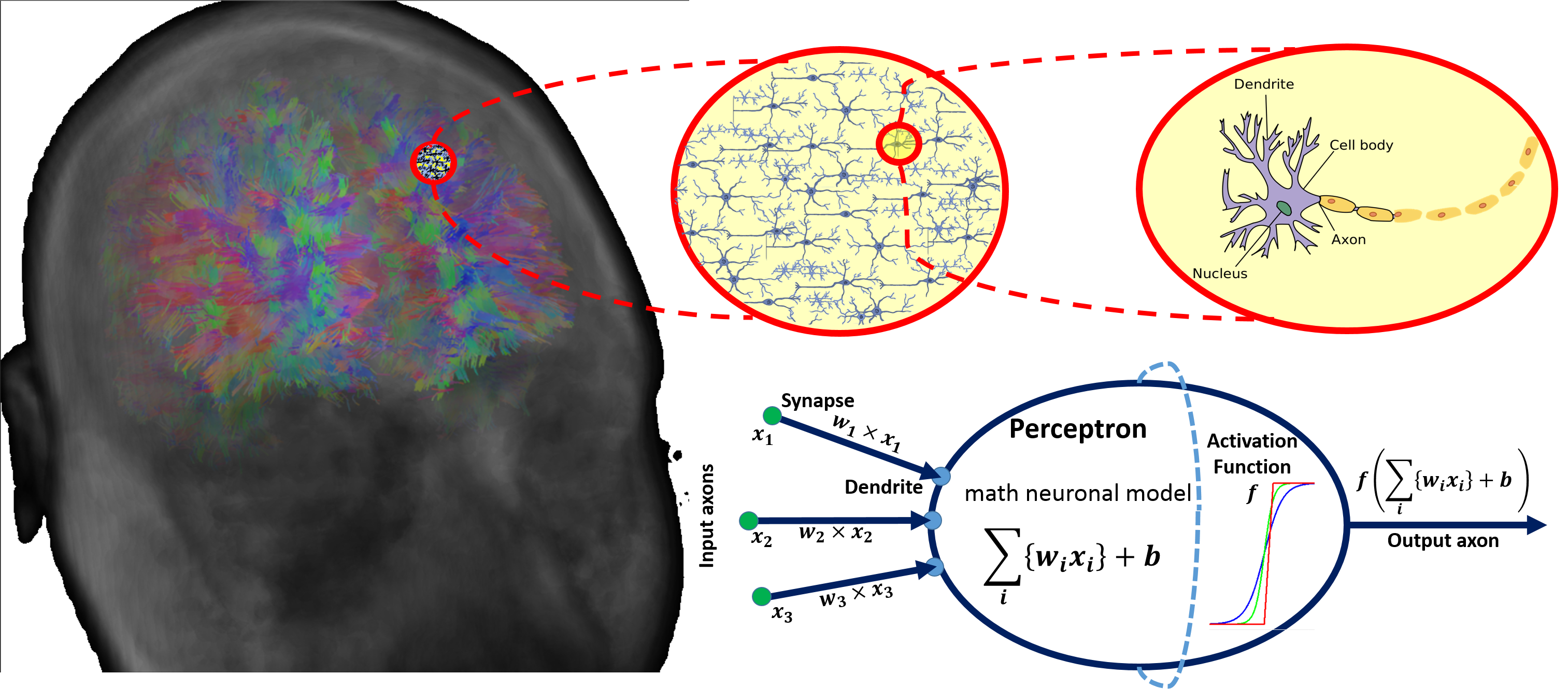#' [![](https://wiki.socr.umich.edu/images/a/a6/DSPA_22_DeepLearning_Fig1.png)](https://wiki.socr.umich.edu/images/a/a6/DSPA_22_DeepLearning_Fig1.png)	
#' 	
#' 	
#' # Simple Neural Net Examples 	
#' 	
#' Before we look at some examples of deep learning algorithms applied to model observed natural phenomena, we will develop a couple of simple networks for computing fundamental Boolean operations.	
#' 	
#' ## Exclusive OR (XOR) Operator	
#' The [exclusive OR (XOR) operator](https://en.wikipedia.org/wiki/Exclusive_or) works as a bivariate binary-outcome function, mapping pairs of false (0) and true (1) values to dichotomous false (0) and true (1) outcomes.	
#' 	
#' We can design a simple two-layer neural network that calculates `XOR`. The **values within each neurons represent its explicit threshold**, which can be normalized so that all neurons utilize the same threshold, typically $1$). The **value labels associated with network connections (edges) represent the weights of the inputs**. When the threshold is not reached, output is $0$, and then the threshold is reached, the output is correspondingly $1$.	
#' 	
#' 	
# install.packages("network")	
library('igraph')	
#define node names	
nodes <- c('X', 'Y',                            # Inputs (0,1)	
           'H_1_1_th1','H_1_2_th2','H_1_3_th1', # Hidden Layer	
           'Z'                                  # Output Layer (0,1)	
           )	
# define node x,y coordinates	
x <- c(rep(0,2), rep(2,3), 4)	
y <- c(c(1.5, 2.5), 1:3, 2)	
##x;y  # print x & y coordinates of all nodes	
	
#define edges	
from <- c('X', 'X', 	
          'Y', 'Y',	
          'H_1_1_th1', 'H_1_2_th2', 'H_1_3_th1',	
          'Z'	
          )	
to <- c('H_1_1_th1', 'H_1_2_th2',	
        'H_1_2_th2', 'H_1_3_th1', 	
        'Z', 'Z', 'Z', 'Z'	
        )	
edge_names <- c(	
        '1', '1',	
        '1', '1',	
        '1', '-2', '1', '1'	
        )	
  	
NodeList <- data.frame(nodes, x ,y)	
EdgeList <- data.frame(from, to, edge_names)	
nn.graph <- graph_from_data_frame(vertices = NodeList, d= EdgeList, directed = TRUE) %>% set_edge_attr("label", value = edge_names)	
# plot(nn.graph)	
	
# See the iGraph specs here: http://kateto.net/networks-r-igraph	
	
col <- rep("gray",length(V(nn.graph))) # input layer	
col[c(3:5)] <- "lightblue"             # hidden layer	
col[6] <- "lightgreen"                 # output layer	
plot(nn.graph, vertex.color=col, vertex.shape="sphere", vertex.size=c(35, 35,   80, 80, 80, 35), edge.label.cex=1.5)	
title(main="XOR Operator")	
mtext("Input Layer: Bivariate (0,1)", side=2, line=-1, col="blue")	
mtext("     Output Layer (XOR)", side=4, line=-2, col="green")	
mtext("Hidden Layers (Neurons)", side=1, line=0, col="gray")	
#' 	
#' 	
#' Let's work out manually the 4 possibilities:	
#' 	
#' InputX|InputY|XOR Output(Z)    	
#' ------|------|-------------   	
#' 0 | 0 |	0	
#' 0 | 1 | 1	
#' 1 | 0 | 1	
#' 1 | 1 | 0	
#' 	
#' We can validate that this network indeed represents an XOR operator by plugging in all four possible input combinations and confirming the expected results at the end.	
#' 	
#' 	
par(mfrow=c(2,2))    # 2 x 2 design	
nodes <- c('X=0', 'Y=0',                        # Inputs 	
           'H_1_1_th1','H_1_2_th2','H_1_3_th1', # Hidden Layer	
           'Z=0'                                # Output Layer (0,1)	
           )	
# define node x,y coordinates	
x <- c(rep(0,2), rep(2,3), 4)	
y <- c(c(1.5, 2.5), 1:3, 2)	
# x;y  # print x & y coordinates of all nodes	
	
######### (0,0)	
#define edges	
from <- c('X=0', 'X=0', 	
          'Y=0', 'Y=0',	
          'H_1_1_th1', 'H_1_2_th2', 'H_1_3_th1',	
          'Z=0'	
          )	
to <- c('H_1_1_th1', 'H_1_2_th2',	
        'H_1_2_th2', 'H_1_3_th1', 	
        'Z=0', 'Z=0', 'Z=0', 'Z=0'	
        )	
edge_names <- c(	
        '1', '1',	
        '1', '1',	
        '1', '-2', '1', '1'	
        )	
  	
NodeList <- data.frame(nodes, x ,y)	
EdgeList <- data.frame(from, to, edge_names)	
nn.graph <- graph_from_data_frame(vertices = NodeList, d= EdgeList, directed = TRUE) %>% set_edge_attr("label", value = edge_names)	
	
col <- rep("gray",length(V(nn.graph))) # input layer	
col[c(3:5)] <- "lightblue"             # hidden layer	
col[6] <- "lightgreen"                 # output layer	
plot(nn.graph, vertex.color=col, vertex.shape="pie", vertex.size=c(30, 30,   40, 40, 40, 30), edge.label.cex=2,	
     edge.arrow.size=0.25)	
title(main="XOR Operator")	
mtext("Input Layer: Bivariate (X=0,Y=0)", side=2,line=-1, col="blue")	
mtext("     Output Layer (XOR), Z=0", side=4, line=-2, col="green")	
mtext("Hidden Layers (Neurons)", side=1, line=0, col="gray")	
	
######### (0,1)	
nodes <- c('X=0', 'Y=1',                        # Inputs 	
           'H_1_1_th1','H_1_2_th2','H_1_3_th1', # Hidden Layer	
           'Z=1'                                # Output Layer (0,1)	
           )	
#define edges	
from <- c('X=0', 'X=0', 	
          'Y=1', 'Y=1',	
          'H_1_1_th1', 'H_1_2_th2', 'H_1_3_th1',	
          'Z=1'	
          )	
to <- c('H_1_1_th1', 'H_1_2_th2',	
        'H_1_2_th2', 'H_1_3_th1', 	
        'Z=1', 'Z=1', 'Z=1',	
        'Z=1'	
        )	
	
NodeList <- data.frame(nodes, x ,y)	
EdgeList <- data.frame(from, to, edge_names)	
nn.graph <- graph_from_data_frame(vertices = NodeList, d= EdgeList, directed = TRUE) %>% set_edge_attr("label", value = edge_names)	
	
col <- rep("gray",length(V(nn.graph))) # input layer	
col[c(3:5)] <- "lightblue"             # hidden layer	
col[6] <- "lightgreen"                 # output layer	
plot(nn.graph, vertex.color=col, vertex.shape="pie", vertex.size=c(30, 30,   40, 40, 40, 30), edge.label.cex=1,	
     edge.arrow.size=0.25)	
title(main="XOR Operator")	
mtext("Input Layer: Bivariate (X=0,Y=1)",side=2,line=-1, col="blue")	
mtext("     Output Layer (XOR), Z=1", side=4, line=-2, col="green")	
mtext("Hidden Layers (Neurons)", side=1, line=0, col="gray")	
	
######### (1,0)	
nodes <- c('X=1', 'Y=0',                        # Inputs 	
           'H_1_1_th1','H_1_2_th2','H_1_3_th1', # Hidden Layer	
           'Z=1'                                # Output Layer (0,1)	
           )	
#define edges	
from <- c('X=1', 'X=1', 	
          'Y=0', 'Y=0',	
          'H_1_1_th1', 'H_1_2_th2', 'H_1_3_th1',	
          'Z=1'	
          )	
to <- c('H_1_1_th1', 'H_1_2_th2',	
        'H_1_2_th2', 'H_1_3_th1', 	
        'Z=1', 'Z=1', 'Z=1',	
        'Z=1'	
        )	
	
NodeList <- data.frame(nodes, x ,y)	
EdgeList <- data.frame(from, to, edge_names)	
nn.graph <- graph_from_data_frame(vertices = NodeList, d= EdgeList, directed = TRUE) %>% set_edge_attr("label", value = edge_names)	
	
col <- rep("gray",length(V(nn.graph))) # input layer	
col[c(3:5)] <- "lightblue"             # hidden layer	
col[6] <- "lightgreen"                 # output layer	
plot(nn.graph, vertex.color=col, vertex.shape="pie", vertex.size=c(30, 30,   40, 40, 40, 30), edge.label.cex=1,	
     edge.arrow.size=0.25)	
title(main="XOR Operator")	
mtext("Input Layer: Bivariate (X=1,Y=0)", side=2,line=-1, col="blue")	
mtext("     Output Layer (XOR), Z=1", side=4, line=-2, col="green")	
mtext("Hidden Layers (Neurons)", side=1, line=0, col="gray")	
	
######### (1,1)	
nodes <- c('X=1', 'Y=1',                        # Inputs 	
           'H_1_1_th1','H_1_2_th2','H_1_3_th1', # Hidden Layer	
           'Z=0'                                # Output Layer (1,1)	
           )	
#define edges	
from <- c('X=1', 'X=1', 	
          'Y=1', 'Y=1',	
          'H_1_1_th1', 'H_1_2_th2', 'H_1_3_th1',	
          'Z=0'	
          )	
to <- c('H_1_1_th1', 'H_1_2_th2',	
        'H_1_2_th2', 'H_1_3_th1', 	
        'Z=0', 'Z=0', 'Z=0',	
        'Z=0'	
        )	
	
NodeList <- data.frame(nodes, x ,y)	
EdgeList <- data.frame(from, to, edge_names)	
nn.graph <- graph_from_data_frame(vertices = NodeList, d= EdgeList, directed = TRUE) %>% set_edge_attr("label", value = edge_names)	
	
col <- rep("gray",length(V(nn.graph))) # input layer	
col[c(3:5)] <- "lightblue"             # hidden layer	
col[6] <- "lightgreen"                 # output layer	
plot(nn.graph, vertex.color=col, vertex.shape="pie", vertex.size=c(30, 30,   40, 40, 40, 30), edge.label.cex=1.5,	
     edge.arrow.size=0.25)	
title(main="XOR Operator")	
mtext("Input Layer: Bivariate (X=1,Y=1)",side=2,line=-1, col="blue")	
mtext("     Output Layer (XOR), Z=0", side=4, line=-2, col="green")	
mtext("Hidden Layers (Neurons)", side=1, line=0, col="gray")	
#' 	
#' 	
#' 	
#' ## NAND Operator	
#' Another binary operator is `NAND` ([negative AND, Sheffer stroke](https://en.wikipedia.org/wiki/NAND_gate)) that produces a false (0) output if and only if both of its operands are true (1), and generates true (1), otherwise. Below is the `NAND` input-output table.	
#' 	
#' InputX|InputY|NAND Output(Z)	
#' ------|------|------------- 	
#' 0 | 0 |	1 	
#' 0 | 1 | 1	
#' 1 | 0 | 1	
#' 1 | 1 | 0	
#' 	
#' Similarly to the `XOR` operator, we can design a one-layer neural network that calculates `NAND`. The **values within each neurons represent its explicit threshold**, which can be normalized so that all neurons utilize the same threshold, typically $1$). The **value labels associated with network connections (edges) represent the weights of the inputs**. When the threshold is not reached, the output is trivial ($0$) and when the threshold is reached, the output is correspondingly $1$. Here is a shorthand analytic expression for the `NAND` calculation:	
#' 	
#' $$NAND(X,Y) = 1.3 - (1\times X + 1\times Y).$$	
#' Check that $NAND(X,Y)=0$ if and only if $X=1$ and $Y=1$, otherwise it equals $1$.	
#' 	
#' 	
# install.packages("network")	
library('igraph')	
#define node names	
nodes <- c('X', 'Y',                            # Inputs (0,1)	
           'H_th=1.3-(X+Y)',            # Hidden Layer	
           'Z'                                  # Output Layer (0,1)	
           )	
# define node x,y coordinates	
x <- c(rep(0,2), 2, 4)	
y <- c(c(1.5, 2.5), 2, 2)	
#x;y  # print x & y coordinates of all nodes	
	
#define edges	
from <- c('X', 'Y', 	
          'H_th=1.3-(X+Y)'	
          )	
to <- c('H_th=1.3-(X+Y)', 'H_th=1.3-(X+Y)',	
        'Z'	
        )	
edge_names <- c(	
        '-1', '-1',	
        '1'	
        )	
  	
NodeList <- data.frame(nodes, x ,y)	
EdgeList <- data.frame(from, to, edge_names)	
nn.graph <- graph_from_data_frame(vertices = NodeList, d= EdgeList, directed = TRUE) %>% set_edge_attr("label", value = edge_names)	
# plot(nn.graph)	
	
# See the iGraph specs here: http://kateto.net/networks-r-igraph	
	
col <- rep("gray",length(V(nn.graph))) # input layer	
col[c(3)] <- "lightblue"             # hidden layer	
col[4] <- "lightgreen"                 # output layer	
plot(nn.graph, vertex.color=col, vertex.shape="sphere", vertex.size=c(35, 35,   80,    35), edge.label.cex=2)	
title(main="NAND Operator")	
mtext("Input Layer: Bivariate (X,Y)", side=2, line=-1, col="blue")	
mtext("     Output Layer (NAND)", side=4, line=-2, col="green")	
mtext("Hidden Layers (Neurons)", side=1, line=0, col="gray")	
#' 	
#' 	
#' ## Complex networks designed using simple building blocks 	
#' 	
#' Observe that stringing some of these primitive networks together, or/and increasing the number of hidden layers, allows us to model problems with exponentially increasing complexity. For instance, constructing a 4-input `NAND` function would simply require repeating several of our 2-input `NAND` operators. This will increase the space of possible outcomes from $2^2$ to $2^4$. Of course, introducing more depth in the **hidden layers** further expands the complexity of the problems that can be modeled using neural nets.	
#' 	
#' You can interactively manipulate the [Google's TensorFlow Deep Neural Network Webapp](https://playground.tensorflow.org) to gain additional intuition and experience with the various components of deep learning networks. 	
#' 	
#' The [ConvnetJS demo provide another hands-on example using 2D classification with 2-layer neural network]( http://cs.stanford.edu/people/karpathy/convnetjs/demo/classify2d.html).	
#' 	
#' # Neural Network Modeling using `Keras`	
#' 	
#' There are many different neural-net and deep-learning frameworks. The table below summarizes some of the main deep learning `R` packages.	
#' 	
#' Package     | Description	
#' ----------  | --------------------------------------------------------------------	
#' nnet 	      |   Feed-forward neural networks using 1 hidden layer	
#' neuralnet 	| 	Training backpropagation neural networks	
#' tensorflow  |   Google TensorFlow used in TensorBoard (see [SOCR UKBB Demo](https://socr.umich.edu/HTML5/SOCR_TensorBoard_UKBB/))	
#' deepnet     |  	Deep learning toolkit	
#' darch       | 	Deep Architectures based on Restricted Boltzmann Machines	
#' rnn         |   Recurrent Neural Networks (RRNs)	
#' rcppDL      |   Multi-layer machine learning methods including dA (Denoising Autoencoder), SdA (Stacked Denoising Autoencoder), RBM (Restricted Boltzmann machine), and DBN (Deep Belief Nets)	
#' deepr       |   DL training, fine-tuning and predicting processes using darch and deepnet	
#' MXNetR 	    | 	Flexible and efficient ML/DL tools utilizing CPU/GPU computing	
#' kerasR      |   RStudio's keras DL implementation wrapping C++/Python executable libraries	
#' Keras       |   Python based neural networks API, connecting Google TensorFlow, Microsoft Cognitive Toolkit (CNTK), and Theano	
#' 	
#' Most DL/ML `R` packages provide interfaces (APIs) to libraries that are build using foundational languages like C/C++ and Java. Most of the Python libraries also act as APIs to lower-level executables compiled for specific platforms (Mac, Linux, PC).	
#' 	
#' The `keras` package uses the `magrittr` package `pipe` operator (`%>%`) to join multiple functions or operators, which streamlines the readability of the script protocol.	
#' 	
#' The `kerasR` package contains analogous functions to the ones in `keras` and utilizes the $\$$ operator to create models. There are parallels between the core `Python` methods and their `keras` counterparts: `compile()` and `keras_compile()`, `fit()` and `keras_fit()`, `predict()` and `keras_predict()`.	
#' 	
#' Below we will demonstrate the utilization of the `Keras` package for deep neural network analytics. This will require installation of `keras` and `TensorFlow` via `R` `devtools::install_github("rstudio/keras")`. See the details about [keras installation here](https://tensorflow.rstudio.com/reference/keras/install_keras/).	
#' 	
#' 	
# devtools::install_github("rstudio/keras")	
library("keras")	
# install_keras()	
	
#install.packages("tensorflow")	
library(tensorflow)	
#install_tensorflow()	
#' 	
#' 	
#' The [`Keras` package](https://keras.rstudio.com/) includes built-in datasets with `load()` functions, e.g., `mnist.load_data()` and `imdb.load_data()`.	
#' 	
#' 	
mnist <- dataset_mnist()	
imdb <- dataset_imdb()	
#' 	
#' 	
#' ## Use-Case: Predicting Titanic Passenger Survival	
#' 	
#' Instead of using the default data provided in the `keras` package, we will utilize one of the datasets on the [DSPA Case-Studies Website](https://umich.instructure.com/courses/38100/files/folder/Case_Studies), can also be loaded much like [we have done before](https://www.socr.umich.edu/people/dinov/courses/DSPA_notes/02_ManagingData.html). Below, we download the [Titanic Passenger Dataset](https://umich.instructure.com/courses/38100/files/folder/data/16_TitanicPassengerSurvivalDataset).	
#' 	
#' 	
library(reshape)	
library(caret)	
dat <- read.csv("https://umich.instructure.com/files/9372716/download?download_frd=1")	
	
# Inspect for missing values (empty or NA):	
dat.miss <- melt(apply(dat[, -2], 2, function(x) sum(is.na(x) | x=="")))	
cbind(row.names(dat.miss)[dat.miss$value>0], dat.miss[dat.miss$value>0,])	
	
# We can exclude the "Cabin" feature which includes 80% missing values. 	
	
# Impute the few missing Embarked values using the most common value (S)	
table(dat$embarked)	
dat$embarked[which(is.na(dat$embarked) | dat$embarked=="")] <- "S"	
	
# Some "fare"" values may represent total cost of group purchases	
# We can derive a new variable "price" representing fare per person	
# Update missing fare value with 0	
dat$fare[which(is.na(dat$fare))] <- 0 	
# calculate ticket Price (Fare per person)	
ticket.count <- aggregate(dat$ticket, by=list(dat$ticket), function(x) sum( !is.na(x) ))	
dat$price <- apply(dat, 1, function(x) as.numeric(x["fare"]) /	
            ticket.count[which(ticket.count[, 1] == x["ticket"]), 2])	
	
# Impute missing prices (price=0) using the median price per passenger class	
pclass.price<-aggregate(dat$price, by = list(dat$pclass), FUN = function(x) median(x, na.rm = T))	
dat[which(dat$price==0), "price"] <- 	
  apply(dat[which(dat$price==0), ] , 1, function(x)	
    pclass.price[pclass.price[, 1]==x["pclass"], 2])	
	
# Define a new variable "ticketcount" coding the number of passengers sharing the same ticket number	
dat$ticketcount <- 	
  apply(dat, 1, function(x) ticket.count[which(ticket.count[, 1] ==	
                                                 x["ticket"]), 2])	
	
# Capture the passenger title	
dat$title <- 	
  regmatches(as.character(dat$name),	
             regexpr("\\,[A-z ]{1,20}\\.", as.character(dat$name)))	
dat$title <-	
  unlist(lapply(dat$title,	
            FUN=function(x) substr(x, 3, nchar(x)-1)))	
table(dat$title)	
	
# Bin the 17 alternative title groups into 4 common 4 titles (factors)	
dat$title[which(dat$title %in% c("Mme", "Mlle"))] <- "Miss"	
dat$title[which(dat$title %in% 	
                  c("Lady", "Ms", "the Countess", "Dona"))] <- "Mrs"	
dat$title[which(dat$title=="Dr" & dat$sex=="female")] <- "Mrs"	
dat$title[which(dat$title=="Dr" & dat$sex=="male")] <- "Mr"	
dat$title[which(dat$title %in% c("Capt", "Col", "Don", 	
                  "Jonkheer", "Major", "Rev", "Sir"))] <- "Mr"	
dat$title <- as.factor(dat$title) 	
table(dat$title)	
	
# Impute missing ages using median age for each title group	
title.age <- aggregate(dat$age, by = list(dat$title), 	
                    FUN = function(x) median(x, na.rm = T))	
dat[is.na(dat$age), "age"] <- apply(dat[is.na(dat$age), ] , 1, 	
              function(x) title.age[title.age[, 1]==x["title"], 2])	
#' 	
#' 	
#' ## EDA/Visualization	
#' We can start by some [simple EDA plots](https://www.socr.umich.edu/people/dinov/courses/DSPA_notes/03_DataVisualization.html), reporting some numerical summaries, examining pairwise correlations, and showing the distributions of some features in this dataset.	
#' 	
#' 	
library(ggplot2)	
summary(dat)	
	
# cols <- c("red","green")[unclass(dat$survived)]	
# 	
# plot(dat$ticketcount, dat$fare, pch=21, cex=1.5,	
#      bg=alpha(cols, 0.4),	
#      xlab="Number of Tickets per Party", ylab="Passenger Fare", 	
#      main="Titanic Passenger Data (TicketCount vs. Fare) Color Coded by Survival")	
# legend("topright", inset=.02, title="Survival",	
#    c("0","1"), fill=c("red", "green"), horiz=F, cex=0.8)	
	
plot_ly(dat, type="scatter")  %>%	
    add_trace(x = ~ticketcount, y=~fare, mode = 'markers', 	
              color = ~as.character(survived), colors=~survived) %>%	
    layout(legend = list(title=list(text='<b> Survival </b>'), orientation = 'h'), 	
           title="Titanic Passenger Data (TicketCount vs. Fare) Color Coded by Survival")	
	
	
# ggplot(dat, aes(x=survived, y=fare, fill=sex)) + 	
#   #geom_dotplot(binaxis='y', stackdir='center',	
#   #               position=position_dodge(1)) +	
#   #scale_fill_manual(values=c("#999999", "#E69F00")) +	
#   geom_violin(trim=FALSE) +	
#   theme(legend.position="top")	
	
	
fig <- dat %>% plot_ly(type = 'violin') 	
fig <- fig %>% add_trace(x = ~survived[dat$survived == '1'], y = ~fare[dat$survived == '1'],	
    legendgroup = 'survived',   scalegroup = 'survived',  name = 'survived',  	
    box = list(visible = T),  meanline = list(visible = T ),  color = I("green")) 	
fig <- fig %>% add_trace(x = ~survived[dat$survived == '0'], y = ~fare[dat$survived == '0'],	
    legendgroup = 'died',   scalegroup = 'died',  name = 'died',  	
    box = list(visible = T),  meanline = list(visible = T ),  color = I("red"))	
fig <- fig %>% layout( xaxis = list(title="Survival"), yaxis = list(title="Fare"),	
                       title='<b> Titanic Passenger Survival vs. Fare </b>', orientation = 'h')	
fig	
	
# library(GGally)	
# ggpairs(dat[ , c("pclass", "age", "sibsp", "parch", 	
#                  "fare", "price", "ticketcount", "survived")], 	
#         aes(colour = as.factor(survived), alpha = 0.4))	
	
dims <- dplyr::select_if(dat, is.numeric)	
dims <- purrr::map2(dims, names(dims), ~list(values=.x, label=.y))	
plot_ly(type = "splom", dimensions = setNames(dims, NULL), showupperhalf = FALSE, 	
        diagonal = list(visible = FALSE) ) %>% 	
  layout( title='<b> Titanic Passengers Pairs-Plots </b>')	
#' 	
#' 	
#' ## Data Preprocessing	
#' 	
#' Before we go into modeling the data, we need to preprocess it, e.g., normalize the numerical values and split it into training and testing sets.	
#' 	
#' 	
dat1 <- dat[ , c("pclass", "age", "sibsp", "parch", "fare", 	
                 "price", "ticketcount", "survived")]	
dat1$pclass <- as.factor(dat1$pclass)	
dat1$age <- as.numeric(dat1$age)	
dat1$sibsp <- as.factor(dat1$sibsp)	
dat1$parch <- as.factor(dat1$parch)	
dat1$fare <- as.numeric(dat1$fare)	
dat1$price <- as.numeric(dat1$price)	
dat1$ticketcount <- as.numeric(dat1$ticketcount)	
dat1$survived <- as.factor(dat1$survived)	
	
# Set the `dimnames` to `NULL`	
# dimnames(dat1) <- NULL	
dim(dat1)	
#' 	
#' 	
#' Use `keras::normalize()` to normalize the numerical data.	
#' 	
#' 	
# devtools::install_github("rstudio/keras")	
# First install Anaconda/Python: https://www.anaconda.com/download/#windows	
# install_keras()	
# reticulate::py_config()	
# library("keras")	
# use_python("C:/Users/Dinov/AppData/Local/Programs/Python/Python37/python.exe")	
# install_keras()	
# install_keras(method = "conda")	
# install_tensorflow()	
library("keras")	
# Normalize the data	
summary(dat1[ , c(2,5,6,7)])	
dat2 <- dat1[ , c(2,5,6,7)]	
dat2 <- as.matrix(dat2)	
dimnames(dat2) <- NULL	
# May be best to avoid normalizing the ordinal variable "ticketcount"	
dat2.norm <- keras::normalize(dat2)	
	
# report the summary`	
summary(dat2.norm)	
colnames(dat2.norm) <- c("age", "fare", "price", "ticketcount")	
#' 	
#' 	
#' Next, we'll partition the raw data into *training* (80%) and *testing* (20%) sets that will be utilized to build the forecasting model (to predict Titanic passenger survival) and assess the model performance, respectively. 	
#' 	
#' 	
train_set_ind <- sample(nrow(dat2.norm), floor(nrow(dat2.norm)*0.8)) # 80:20 plot training:testing	
train_dat2.X <- dat2.norm[train_set_ind, ]	
train_dat2.Y <- dat1[train_set_ind , 8]  # Outcome "survived" column:8	
	
test_dat2.X <- dat2.norm[-train_set_ind, ]	
test_dat2.Y <- dat1[-train_set_ind , 8]  # Outcome "survived" column:8	
	
# double check the size/dimensions of the training and testing data (predictors and responses)	
dim(train_dat2.X); length(train_dat2.Y); dim(test_dat2.X); length(test_dat2.Y)	
#' 	
#' 	
#' ## Keras Modeling	
#' 	
#' For *multi-class classification problems* via NN modeling, the `keras::to_categorical()` function allows us to transform the outcome attribute from a vector of class labels to a matrix of Boolean features, one for each class label. In this case, we have a bivariate (binary classification), passenger survival indicator.	
#' 	
#' Keras modeling starts with first initializing a sequential model using the `keras::keras_model_sequential()` function. 	
#' 	
#' We will try to predict the passenger survival using a fully-connected multi-layer perceptron NN. We will need to choose an activation function, e.g., `relu`, `sigmoid`. A rectifier activation function (relu) may be used in a hidden layer and a `softmax` activation function may be used in the final output layer so that the outputs represent (posterior) probabilities between 0 and 1, corresponding to the odds of survival. In the first layer, we can specify 8 hidden nodes (`units`), an `input_shape` of 4, to reflect the 4 features in the training data *age*, *fare*, *price*, *ticketcount*, and the output layer with 2 output values, one for each of the survival categories. We can also inspect the structure of the NN model using:	
#' 	
#'   - `summary()`: print a summary representation of your model,	
#'   - `get_config()`: return a list that contains the configuration of the model,	
#'   - `get_layer()`: return the layer configuration,	
#'   - `$layers`: NN model attribute retrieves a flattened list of the model's layers,	
#'   - `$inputs`: NN model attribute listing the input tensors,	
#'   - `$outputs`: NN model attribute retrieve the output tensors.	
#' 	
#' 	
model.1 <- keras_model_sequential() 	
	
# Add layers to the model	
model.1 %>% 	
    layer_dense(units = 8, activation = 'relu', input_shape = c(4)) %>% 	
    layer_dense(units = 2, activation = 'softmax')	
	
# NN model summary	
summary(model.1)	
# Report model configuration	
get_config(model.1)	
# report layer configuration	
get_layer(model.1, index = 1)	
# Report model layers	
model.1$layers	
# List the input tensors	
model.1$inputs	
# List the output tensors	
model.1$outputs	
#' 	
#' 	
#' Once the model architecture is specified, we need to estimate (fit) the NN model using the `training` data. The adaptive momentum (`ADAM`) optimizer along with `categorical_crossentropy` objective function may be used to **compile** the NN model. Specifying `accuracy` as a metrics argument allows us to inspect the quality of the NN model fit during the training phase (training data validation). The *optimizer* and the *objective* (loss) function are the pair of require arguments for model compilation. 	
#' 	
#' In addition to *ADAM*, alternative optimization algorithms include Stochastic Gradient Descent (*SGD*) and Root Mean Square proportion (*RMSprop*). ADAM is essentially RMSprop with momentum whereas NADAM is ADAM RMSprop with Nesterov momentum. Following the selection of the optimization algorithm, we need to tune the model parameters, e.g., learning rate or momentum. Choosing an appropriate objective function function depends on the classification or regression forecasting task, e.g., regression prediction (continuous outcomes) usually utilize Mean Squared Error (*MSE*), whereas multi-class classification problems use *categorical_crossentropy* loss function and binary classification problems commonly use *binary_crossentropy* loss function.	
#' 	
#' 	
# "Compile"" the model	
model.1 %>% compile(	
     loss = 'binary_crossentropy',	
     optimizer = 'adam',	
     metrics = 'accuracy'	
 )	
#' 	
#' 	
#' ## NN Model Fitting	
#' 	
#' The next step fits the NN model (`model.1`) to the training data using 200 epochs, or iterations over all the samples in `train_dat2.X` (predictors) and `train_dat2.Y` (outcomes), in batches of 10 samples. This process trains the model a specified number of epochs (iterations or exposures) on the training data. One epoch is a single pass through the whole training set followed by comparing the model prediction results against the verification labels. The batch size defines the number of samples being propagated through the network at ones (as a batch). 	
#' 	
#' 	
# convert the labels to categorical values	
train_dat2.Y <- to_categorical(train_dat2.Y)	
test_dat2.Y <- to_categorical(test_dat2.Y)	
	
# Fit the model & Store the fitting history	
track.model.1 <- model.1 %>% fit(	
     train_dat2.X, 	
     train_dat2.Y, 	
     epochs = 200, 	
     batch_size = 10, 	
     validation_split = 0.2	
 )	
#' 	
#' 	
#' ## Convolutional Neural Networks (CNNs)	
#' Convolutional Neural Networks represent a specific type of Deep Learning algorithms that incorporate the topological, geometric, spatial and temporal structure of the input data (generally images) and assign importance by learning the weights and biases of the (image) intensities associated with the objects or affinities present in the data. These importance features are then utilized to differentiate between datasets (images) or components within the data (structure and objects in images). CNNs require less pre-processing compared to other DL classification algorithms, which may depend on manually-specified filters. CNNs tend to learn these filters by iteratively extrapolating multi-resolution characteristics in the data objects by convolution methods. See the [DSPA Appendix for the mathematical operation convolution and its applications in image processing](https://www.socr.umich.edu/people/dinov/courses/DSPA_notes/DSPA_Appendix_6_ImageFilteringSpectralProcessing.html).	
#' 	
#' Recall that one may attempt to learn the features of an image (or a higher dimensional tensor) by flattening the image array (matrix/tensor) into a 1D vector. This vectorization works well if there are no spatiotemporal dependencies in the data. Most of the time, there are such image intensity correlations that can’t be ignored. The CNN architecture facilitates a mechanism to better model the intrinsic image affinities, reduce the number of DNN parameters, and produce more reliable predictions. Many images are represented as tensors whose modes (dimensions) encode spatial, temporal, color-channel, and other information about the observed image intensity. For instance, an RGB image of size $1,000 \times 1,000=10^6$ pixels, may require 3MB of memory/storage. A CNN learns to encode the image into a higher-dimensional multispectral hierarchical tensor encoding the intrinsic image characteristics that can lead to easy classification of similar images or generation of synthetic images. For instance, ignoring the color-channels and using a stride=10, convoluting the original image of dimension with a kernel of size $10\times 10$ would yield another (smoother) lower-resolution image of size $100\times 100$, encoding the convolved features. 	
#' 	
#' The convolution process aims to extract the high-level features such as edges, borders, and contrasts from the input image. CNNs involve both convolutional and dense layer. Much like the [Fourier transform](https://www.socr.umich.edu/TCIU/HTMLs/Chapter3_Kime_Phase_Problem.html), the first convolutional layer captures low-level features such as edges, color, gradient orientation, etc. Subsequent layers progressively add higher-level details and the entire CNN encodes holistically the understanding of the input image structure.	
#' 	
#' Convolution, de-convolution (the reverse process) and padding reduce or increase the image dimensionality. 	
#' Most CNNs mix *convolutional layers* with *pooling layers*. The latter are responsible for reducing the spatial size of the convolved features, which decreases the computational data processing demand. Pooling may be implemented as *Max Pooling* or *Average Pooling*. Max-pooling takes an image patch defined by the kernel and returns the maximum intensity value. It performs noise-suppression as it decimates noisy pixel intensities, denoises the image, and reduces the image dimensions. Average-pooling returns the average of all intensity values covered by the image-kernel and reduces the image dimension.	
#' 	
#' Jointly, the convolutional and the pooling processes form the CNN $i$-th layer and the number of layers may reflect the ANN complexity. Fully connected layers are typically added to the ANN architecture to enhance the classification, prediction, or regression performance of DL model. Fully-connected layers provide mechanism to learn non-linear associations and non-affine characteristics of high-level features captured as outputs of the convolutional layers. 	
#' 	
#' ## Model EDA	
#' 	
#' We can visualize the model fitting process using `keras::plot()` jointly depicting the loss of the objective function and the accuracy of the model, across epochs. Alternatively, we can split the pair of plots - one for the *model loss* and the other one for the *model accuracy*. The $\$$ operator is used to access the tensor data and plot it step-by-step. A sign of overfitting may be an accuracy (on training data) that keeps improving while the accuracy (on the validation data) worsens. This may be in indication that the NN model starts to *learn* noise in the data instead of learning real patterns or affinities in the data. While the accuracy trends of both datasets are rising towards the final epochs, this may indicate that the model is still in the process of learning on the training dataset (and we can increase the number of epochs).	
#' 	
#' 	
# Plot the history	
# plot(track.model.1)	
# 	
# # NN model loss on the training data	
# plot(track.model.1$metrics$loss, main="Model 1 Loss", 	
#      xlab = "Epoch", ylab="Loss", col="green", type="l", ylim=c(0.54, 0.6))	
# 	
# # NN model loss of the 20% validation data	
# lines(track.model.1$metrics$val_loss, col="blue", type="l")	
# 	
# # Add legend	
# legend("right", c("train", "test"), col=c("green", "blue"), lty=c(1,1))	
# 	
# # Plot the accuracy of the training data 	
# plot(track.model.1$metrics$acc, main="Model 1 Accuracy", 	
#      xlab = "Epoch", ylab="Accuracy", col="blue", type="l", ylim=c(0.65, 0.75))	
# 	
# # Plot the accuracy of the validation data	
# lines(track.model.1$metrics$val_acc, col="green")	
# 	
# # Add Legend	
# legend("bottom", c("Training", "Testing"), col=c("blue", "green"), lty=c(1,1))	
	
## plot_ly	
epochs <- 200	
time <- 1:epochs	
hist_df <- data.frame(time=time, loss=track.model.1$metrics$loss, acc=track.model.1$metrics$acc,	
                      valid_loss=track.model.1$metrics$val_loss, valid_acc=track.model.1$metrics$val_acc)	
	
plot_ly(hist_df, x = ~time)  %>%	
  add_trace(y = ~loss, name = 'training loss', mode = 'lines') %>%	
  add_trace(y = ~acc, name = 'training accuracy', mode = 'lines+markers') %>%	
  add_trace(y = ~valid_loss, name = 'validation loss',mode = 'lines+markers') %>%	
  add_trace(y = ~valid_acc, name = 'validation accuracy', mode = 'lines+markers') %>% 	
  layout(legend = list(orientation = 'h'))	
#' 	
#' 	
#' ## Passenger Survival Forecasting using New Data	
#' 	
#' Once the model is fit, we can use it to predict the survival of passengers using the testing data, `test_dat2.X`. As we have seen before `predict()` provides this functionality. Finally, we can evaluate the performance of the NN model by comparing the predicted class labels and `test_dat2.Y` using `table()` or `confusionMatrix()`.	
#' 	
#' 	
# Predict the classes for the test data	
predict.survival <- model.1 %>% predict_classes(test_dat2.X, batch_size = 30)	
	
# Confusion matrix	
test_dat2.Y <- dat1[-train_set_ind , 8]	
table(test_dat2.Y, predict.survival)	
caret::confusionMatrix(test_dat2.Y, as.factor(predict.survival))	
#' 	
#' 	
#' We can also utilize the `evaluate()` function to assess the model quality using testing data.	
#' 	
#' 	
# Evaluate on test data and labels	
test_dat2.Y <- to_categorical(test_dat2.Y)	
model1.qual <- model.1 %>% evaluate(test_dat2.X, test_dat2.Y, batch_size = 30)	
print(model1.qual)	
#' 	
#' 	
#' ## Fine-tuning the NN Model	
#' 	
#' The main NN model parameters we can adjust to improve the model quality include:	
#' 	
#'  - the *number of layers* 	
#'  - the *number of nodes* within layers (*hidden units*).	
#'  - the *number of epochs* 	
#'  - the *batch size*.	
#'   	
#' Models can be improved by adding additional layers, increasing the number of hidden units, and by tuning the optimization parameters in `compile()`. Let's first try to add another layer to the N model.	
#' 	
#' 	
# Initialize the sequential model	
model.2 <- keras_model_sequential() 	
	
# Add layers to model	
model.2 %>% 	
    layer_dense(units = 8, activation = 'relu', input_shape = c(4)) %>% 	
    layer_dense(units = 6, activation = 'relu') %>% 	
    layer_dense(units = 2, activation = 'softmax')	
	
# Compile the model	
model.2 %>% compile(	
     loss = 'binary_crossentropy',	
     optimizer = 'adam',	
     metrics = 'accuracy'	
 )	
	
# Fit NN model to training data & Save the training history	
track.model.2 <- model.2 %>% fit(	
     train_dat2.X, 	
     train_dat2.Y, 	
     epochs = 200, 	
     batch_size = 10, 	
     validation_split = 0.2	
 )	
	
# Evaluate the model	
model2.qual <- model.2 %>% evaluate(test_dat2.X, test_dat2.Y, batch_size = 30)	
print(model2.qual)	
	
# EDA on the loss and accuracy metrics of this model.2	
# Plot the history	
# plot(track.model.2)	
# 	
# # NN model loss on the training data	
# plot(track.model.2$metrics$loss, main="Model Loss", 	
#      xlab = "Epoch", ylab="Loss", col="green", type="l", ylim=c(0.54, 0.6))	
# 	
# # NN model loss of the 20% validation data	
# lines(track.model.2$metrics$val_loss, col="blue", type="l")	
# 	
# # Add legend	
# legend("right", c("Training", "Testing"), col=c("green", "blue"), lty=c(1,1))	
# 	
# # Plot the accuracy of the training data 	
# plot(track.model.2$metrics$acc, main="Model 2 (Extra Layer) Accuracy", 	
#      xlab = "Epoch", ylab="Accuracy", col="blue", type="l", ylim=c(0.65, 0.76))	
# 	
# # Plot the accuracy of the validation data	
# lines(track.model.2$metrics$val_acc, col="green")	
# 	
# # Add Legend	
# legend("top", c("Training", "Testing"), col=c("blue", "green"), lty=c(1,1))	
	
## plot_ly	
epochs <- 200	
time <- 1:epochs	
hist_df2 <- data.frame(time=time, loss=track.model.2$metrics$loss, acc=track.model.2$metrics$acc,	
                      valid_loss=track.model.2$metrics$val_loss, valid_acc=track.model.2$metrics$val_acc)	
	
plot_ly(hist_df2, x = ~time)  %>%	
  add_trace(y = ~loss, name = 'training loss', mode = 'lines') %>%	
  add_trace(y = ~acc, name = 'training accuracy', mode = 'lines+markers') %>%	
  add_trace(y = ~valid_loss, name = 'validation loss',mode = 'lines+markers') %>%	
  add_trace(y = ~valid_acc, name = 'validation accuracy', mode = 'lines+markers') %>% 	
  layout(legend = list(orientation = 'h'))	
#' 	
#' 	
#' Next we can examine the effects of adding more *hidden units* to the NN model.	
#' 	
#' 	
# Initialize a sequential model	
model.3 <- keras_model_sequential() 	
	
# Add layers and Node-Units to model	
model.3 %>% 	
    layer_dense(units = 30, activation = 'relu', input_shape = c(4)) %>% 	
    layer_dense(units = 15, activation = 'relu') %>% 	
    layer_dense(units = 2, activation = 'softmax')	
	
# Compile the model	
model.3 %>% compile(	
     loss = 'binary_crossentropy',	
     optimizer = 'adam',	
     metrics = 'accuracy'	
 )	
	
# Fit NN model to training data & Save the training history	
track.model.3 <- model.3 %>% fit(	
     train_dat2.X, 	
     train_dat2.Y, 	
     epochs = 200, 	
     batch_size = 10, 	
     validation_split = 0.2	
 )	
	
# Evaluate the model	
model3.qual <- model.3 %>% evaluate(test_dat2.X, test_dat2.Y, batch_size = 30)	
print(model3.qual)	
	
# EDA on the loss and accuracy metrics of this model.2	
# Plot the history	
# plot(track.model.3)	
# 	
# # NN model loss on the training data	
# plot(track.model.3$metrics$loss, main="Model Loss", 	
#      xlab = "Epoch", ylab="Loss", col="green", type="l", ylim=c(0.54, 0.7))	
# 	
# # NN model loss of the 20% validation data	
# lines(track.model.3$metrics$val_loss, col="blue", type="l")	
# 	
# # Add legend	
# legend("top", c("Training", "testing"), col=c("green", "blue"), lty=c(1,1))	
# 	
# # Plot the accuracy of the training data 	
# plot(track.model.3$metrics$acc, main="Model 3 (Extra Layer/More Hidden Units)", 	
#      xlab = "Epoch", ylab="Accuracy", col="blue", type="l", ylim=c(0.65, 0.76))	
# 	
# # Plot the accuracy of the validation data	
# lines(track.model.3$metrics$val_acc, col="green")	
# 	
# # Add Legend	
# legend("top", c("Training", "Testing"), col=c("blue", "green"), lty=c(1,1))	
	
## plot_ly	
epochs <- 200	
time <- 1:epochs	
hist_df3 <- data.frame(time=time, loss=track.model.3$metrics$loss, acc=track.model.3$metrics$acc,	
                      valid_loss=track.model.3$metrics$val_loss, valid_acc=track.model.3$metrics$val_acc)	
	
plot_ly(hist_df3, x = ~time)  %>%	
  add_trace(y = ~loss, name = 'training loss', mode = 'lines') %>%	
  add_trace(y = ~acc, name = 'training accuracy', mode = 'lines+markers') %>%	
  add_trace(y = ~valid_loss, name = 'validation loss',mode = 'lines+markers') %>%	
  add_trace(y = ~valid_acc, name = 'validation accuracy', mode = 'lines+markers') %>% 	
  layout(legend = list(orientation = 'h'))	
#' 	
#' 	
#' Finally, we can attempt to fine-tune the optimization parameters provided to the `compile()` function. For instance, we can experiment with alternative optimization algorithms, like the Stochastic Gradient Descent (SGD), `optimizer_sgd()`, and adjust the *learning rate*, `lr`. Specifying alternative learning rate to train the NN, typically 10-fold increase or decrease, to trade accuracy, speed of convergence, and avoiding local minima.	
#' 	
#' 	
model.4 <- keras_model_sequential() 	
	
# Add layers and Node-Units to model	
model.4 %>% 	
    layer_dense(units = 30, activation = 'relu', input_shape = c(4)) %>% 	
    layer_dense(units = 15, activation = 'relu') %>% 	
    layer_dense(units = 2, activation = 'softmax')	
	
# Define an optimizer	
SGD <- optimizer_sgd(lr = 0.001)	
	
# Compile the model	
model.4 %>% compile(	
    optimizer=SGD, 	
    loss = 'binary_crossentropy',	
    metrics = 'accuracy'	
 )	
	
# Fit NN model to training data & Save the training history	
set.seed(1234)	
track.model.4 <- model.4 %>% fit(	
     train_dat2.X, 	
     train_dat2.Y, 	
     epochs = 200, 	
     batch_size = 10, 	
     validation_split = 0.1	
 )	
	
# Evaluate the model	
model4.qual <- model.4 %>% evaluate(test_dat2.X, test_dat2.Y, batch_size = 30)	
print(model4.qual)	
	
# EDA on the loss and accuracy metrics of this model.2	
# Plot the history	
# plot(track.model.4)	
# 	
# # NN model loss on the training data	
# plot(track.model.4$metrics$loss, main="Model 4 Loss", 	
#      xlab = "Epoch", ylab="Loss", col="green", type="l", ylim=c(0.54, 0.7))	
# 	
# # NN model loss of the 20% validation data	
# lines(track.model.4$metrics$val_loss, col="blue", type="l")	
# 	
# # Add legend	
# legend("top", c("Training", "Testing"), col=c("green", "blue"), lty=c(1,1))	
# 	
# # Plot the accuracy of the training data 	
# plot(track.model.4$metrics$acc, main="Model 4 (Extra Layer/More Hidden Units/SGD)", 	
#      xlab = "Epoch", ylab="Accuracy", col="blue", type="l", ylim=c(0.65, 0.76))	
# 	
# # Plot the accuracy of the validation data	
# lines(track.model.4$metrics$val_acc, col="green")	
# 	
# # Add Legend	
# legend("top", c("Training", "Testing"), col=c("blue", "green"), lty=c(1,1))	
	
epochs <- 200	
time <- 1:epochs	
hist_df4 <- data.frame(time=time, loss=track.model.4$metrics$loss, acc=track.model.4$metrics$acc,	
                      valid_loss=track.model.4$metrics$val_loss, valid_acc=track.model.4$metrics$val_acc)	
	
plot_ly(hist_df3, x = ~time)  %>%	
  add_trace(y = ~loss, name = 'training loss', mode = 'lines') %>%	
  add_trace(y = ~acc, name = 'training accuracy', mode = 'lines+markers') %>%	
  add_trace(y = ~valid_loss, name = 'validation loss',mode = 'lines+markers') %>%	
  add_trace(y = ~valid_acc, name = 'validation accuracy', mode = 'lines+markers') %>% 	
  layout(legend = list(orientation = 'h'))	
	
#' 	
#' 	
#' ## Model Export and Import	
#' 	
#' Intermediate and final NN models may be saved, (re)loaded, and exported using of `save_model_hdf5()` and `load_model_hdf5()` based on the [HDF5 file format (h5)](https://support.hdfgroup.org/HDF5/whatishdf5.html). We can operate on *complete models* on just on the *model weights*. the models can also be exported in [JSON](https://www.json.org) or [YAML](http://yaml.org) formats using `model_to_json()` and `model_to_yaml()`, and their load counterparts `model_from_json()` and `model_from yaml()`.	
#'   	
#' 	
save_model_hdf5(model.4, "model.4.h5")	
model.new <- load_model_hdf5("model.4.h5")	
	
save_model_weights_hdf5("model_weights.h5")	
model.old %>% load_model_weights_hdf5("model_weights.h5")	
	
json_string <- model_to_json(model.old)	
model.new <- model_from_json(json_string)	
	
yaml_string <- model_to_yaml(model.old)	
model.new <- model_from_yaml(yaml_string)	
#' 	
#' 	
#' 	
#' 	
library(keras)	
	
# get info about local version of Python installation	
reticulate::py_config()	
# The first time you run this install Pillow!	
# tensorflow::install_tensorflow(extra_packages='pillow')	
	
# load the image	
download.file("https://upload.wikimedia.org/wikipedia/commons/2/23/Lake_mapourika_NZ.jpeg", paste(getwd(),"results/image.png", sep="/"), mode = 'wb')	
img <- image_load(paste(getwd(),"results/image.png", sep="/"), target_size = c(224,224))	
	
# Preprocess input image	
x <- image_to_array(img)	
# ensure we have a 4d tensor with single element in the batch dimension,	
# the preprocess the input for prediction using resnet50	
x <- array_reshape(x, c(1, dim(x)))	
x <- imagenet_preprocess_input(x)	
	
# Specify and compare Predictions based on different Pre-trained Models	
# Model 1: resnet50	
model_resnet50 <- application_resnet50(weights = 'imagenet')	
	
# make predictions then decode and print them	
preds_resnet50 <- model_resnet50 %>% predict(x)	
imagenet_decode_predictions(preds_resnet50, top = 10)	
	
# Model2: VGG19	
model_vgg19 <- application_vgg19(weights = 'imagenet')	
preds_vgg19 <- model_vgg19 %>% predict(x)	
imagenet_decode_predictions(preds_vgg19, top = 10)[[1]]	
	
# Model 3: VGG16	
model_vgg16 <- application_vgg16(weights = 'imagenet')	
preds_vgg16 <- model_vgg16 %>% predict(x)	
imagenet_decode_predictions(preds_vgg16, top = 10)[[1]]	
#' 	
#' 	
#' 	
#' # Classification examples	
#' 	
#' ## Sonar data example	
#' 	
#' Let's load the `mlbench` packages which includes a [Sonar data](https://www.rdocumentation.org/packages/mlbench/versions/2.1-1/topics/Sonar) `mlbench::Sonar` containing information about sonar signals bouncing off a metal cylinder or a roughly cylindrical rock. Each of 208 patterns includes a set of 60 numbers (features) in the range 0.0 to 1.0, and a label M (metal) or R (rock). Each feature represents the energy within a particular frequency band, integrated over a certain period of time. The M and R labels associated with each observation classify the record as rock or mine (metal) cylinder. The numbers in the labels are in increasing order of aspect angle, but they do not encode the angle directly. 	
#' 	
#' 	
library(mlbench)	
	
data(Sonar, package="mlbench")	
	
table(Sonar[,61])	
	
Sonar[,61] = as.numeric(Sonar[,61])-1 # R = "1", "M" = "0"	
set.seed(123)	
train.ind = sample(1:nrow(Sonar),0.7*nrow(Sonar))	
	
train.x = data.matrix(Sonar[train.ind, 1:60])	
train.y = Sonar[train.ind, 61]	
test.x = data.matrix(Sonar[-train.ind, 1:60])	
test.y = Sonar[-train.ind, 61]	
#' 	
#' 	
#' Let's start by using a **multi-layer perceptron** as a classifier using a general multi-layer neural network that can be utilized to do classification or regression modeling. It relies on the following parameters:	
#' 	
#' * Training data and labels	
#' * Number of hidden nodes in each hidden layers	
#' * Number of nodes in the output layer	
#' * Type of activation	
#' * Type of output loss	
#' 	
#' Here is one example using the *training* and *testing* data we defined above:	
#' 	
#' 	
library(plotly)	
dim(train.x)  # [1] 145  60	
dim(test.x)   # [1] 63 60	
	
model <- keras_model_sequential() 	
	
model %>% 	
  layer_dense(units = 256, activation = 'relu', input_shape = ncol(train.x)) %>% 	
  layer_dropout(rate = 0.4) %>% 	
  layer_dense(units = 128, activation = 'relu') %>%	
  layer_dropout(rate = 0.3) %>%	
  layer_dense(units = 2, activation = 'sigmoid')	
	
model %>% compile(	
  loss = 'binary_crossentropy',	
  optimizer = 'adam',	
  metrics = c('accuracy')	
)	
	
one_hot_labels <- to_categorical(train.y, num_classes = 2)	
	
# Train the model, iterating on the data in batches of 25 samples	
history <- model %>% fit(	
  train.x, one_hot_labels, 	
  epochs = 100, 	
  batch_size = 5,	
  validation_split = 0.3	
)	
 	
# Evaluate model	
metrics <- model %>% evaluate(test.x, to_categorical(test.y, num_classes = 2))	
metrics	
	
epochs <- 100	
time <- 1:epochs	
hist_df <- data.frame(time=time, loss=history$metrics$loss, acc=history$metrics$accuracy,	
                      valid_loss=history$metrics$val_loss, valid_acc=history$metrics$val_accuracy)	
	
plot_ly(hist_df, x = ~time)  %>%	
  add_trace(y = ~loss, name = 'training loss', mode = 'lines') %>%	
  add_trace(y = ~acc, name = 'training accuracy', mode = 'lines+markers') %>%	
  add_trace(y = ~valid_loss, name = 'validation loss',mode = 'lines+markers') %>%	
  add_trace(y = ~valid_acc, name = 'validation accuracy', mode = 'lines+markers') %>% 	
  layout(legend = list(orientation = 'h'))	
	
# Finally prediction of binary class labels and Confusion Matrix	
predictions <- model %>% predict_classes(test.x)	
	
# We can also inspect the corresponding probabilities of the automated binary classification labels	
prediction_probabilities <- model %>% predict_proba(test.x)	
	
table(factor(predictions),factor(test.y))	
#' 	
#' 	
#' *Note* that you may need to specify `crossval::confusionMatrix()`, in case you also have the `caret` package loaded, as `caret` also has a function called `confusionMatrix()`.	
#' 	
#' 	
library("crossval")	
diagnosticErrors(crossval::confusionMatrix(predictions,test.y, negative = 0))	
#' 	
#' 	
#' We can plot the ROC curve and calculate the AUC (Area under the curve). Specifically, we will show computing the *area under the curve (AUC)* and draw the *receiver operating characteristic (ROC)* curve. Assuming 'positive' ranks higher than 'negative', the [AUC](https://en.wikipedia.org/wiki/Receiver_operating_characteristic#Area_under_the_curve) quantifies the probability that a classifier will rank a randomly chosen positive instance higher than a randomly chosen negative instance. $0\leq AUC\leq 1$ and (bad) *uninformative classifier* yields $AUC=0.5$, whereas $AUC\to 1^-$ suggests a perfect classifier.	
#' 	
#' 	
# install.packages("pROC"); install.packages("plotROC"); install.packages("reshape2")	
library(pROC); library(plotROC); library(reshape2); 	
# compute AUC	
get_roc = function(preds){	
  roc_obj <- roc(test.y, preds, quiet=TRUE)	
  auc(roc_obj)	
}	
get_roc(predictions)	
	
#plot roc	
dt <- data.frame(test.y, predictions)	
colnames(dt) <- c("class","scored.probability")	
	
# basicplot <- ggplot(dt, aes(d = class, m = scored.probability)) + 	
#   geom_roc(labels = FALSE, size = 0.5, alpha.line = 0.6, linejoin = "mitre") +  	
#   theme_bw() + coord_fixed(ratio = 1) + style_roc() + ggtitle("ROC CURVE")+	
#   ggplot2::annotate("rect", xmin = 0.4, xmax = 0.9, ymin = 0.1, ymax = 0.5,	
#            alpha = 0.2)+	
#   ggplot2::annotate("text", x = 0.65, y = 0.32, size = 3,	
#            label = paste0("AUC: ", round(get_roc(predictions)[[1]], 3)))	
# basicplot	
	
# Compute the AUC and draw the ROC curve	
roc_curve <- function(df) {	
  x <- c()	
  y <- c()	
  true_class = df[, "class"]	
  probabilities = df[, "scored.probability"]	
  thresholds = seq(0, 1, 0.01)	
  rx <- 0	
  ry <- 0	
  for (threshold in thresholds) {	
    predicted_class <- c()	
    for (val in probabilities) {	
      if (val > threshold) {	
        predicted_class <- c(predicted_class, 1)	
      }	
      else { predicted_class <- c(predicted_class, 0)   }	
    }	
    df2 <- as.data.frame(cbind(true_class, predicted_class))	
    TP <- nrow(filter(df2, true_class == 1 & predicted_class == 1))	
    TN <- nrow(filter(df2, true_class == 0 & predicted_class == 0))	
    FP <- nrow(filter(df2, true_class == 0 & predicted_class == 1))	
    FN <- nrow(filter(df2, true_class == 1 & predicted_class == 0))	
    specm1 <- 1 - ((TN) / (TN + FP))	
    sens <- (TP) / (TP + FN)	
    x <- append(x, specm1)	
    y <- append(y, sens)	
  }	
  dfr <- as.data.frame(cbind(x, y))	
  plot_ly(dfr, x = ~ x, y = ~ y, type = 'scatter', mode = 'lines') %>%	
    layout(title = paste0("ROC Curve and AUC"), annotations = list(	
        text = paste0("Area Under Curve = ", round(get_roc(predictions)[[1]], 3)),	
        x = 0.75, y = 0.25, showarrow = FALSE),	
      xaxis = list(showgrid = FALSE, title = "1-Specificity (false positive rate)"),	
      yaxis = list(showgrid = FALSE, title = "Sensitivity (true positive rate)"),	
      legend = list(orientation = 'h')	
    ) 	
}	
roc_curve(data.frame(class=test.y, scored.probability=prediction_probabilities[,2]))	
#' 	
#' 	
#' # Case-Studies	
#' 	
#' Let's demonstrate deep neural network regression-modeling and classification-prediction using several biomedical case-studies.	
#' 	
#' ## Schizophrenia Neuroimaging Study	
#' 	
#' [Here is the SOCR Schizo Data](http://wiki.stat.ucla.edu/socr/index.php/SOCR_Data_Oct2009_ID_NI).	
#' 	
#' 	
library("XML"); library("xml2")	
library("rvest");	
	
# Schizophrenia Data	
# UCLA Data is available here: 	
# wiki_url <- read_html("http://wiki.stat.ucla.edu/socr/index.php/SOCR_Data_Oct2009_ID_NI")	
# html_nodes(wiki_url, "#content")	
# SchizoData<- html_table(html_nodes(wiki_url, "table")[[2]])	
# UMich Data is available here	
wiki_url <- read_html("https://wiki.socr.umich.edu/index.php/SOCR_Data_Oct2009_ID_NI")	
html_nodes(wiki_url, "#content")	
SchizoData<- html_table(html_nodes(wiki_url, "table")[[1]])	
	
# View (SchizoData): Select an outcome response "DX"(3), "FS_IQ" (5)	
set.seed(1234)	
test.ind = sample(1:63, 10, replace = F)  # select 10/63 of cases for testing, train on remaining (63-10)/63 cases	
train.x = scale(data.matrix(SchizoData[-test.ind, c(2, 4:9)])) #, 11:66)]) # exclude outcome	
train.y = ifelse(SchizoData[-test.ind, 3] < 2, 1, 2) # Binarize the outcome, Controls=1	
test.x = scale(data.matrix(SchizoData[test.ind, c(2, 4:9)])) #, 11:66)])	
test.y = ifelse(SchizoData[test.ind, 3] < 2, 1, 2)	
	
# View(data.frame(test.x, test.y))	
# View(data.frame(train.x, train.y))	
	
model <- keras_model_sequential() 	
	
model %>% 	
  layer_dense(units = 256, activation = 'relu', input_shape = ncol(train.x)) %>% 	
  layer_dropout(rate = 0.4) %>% 	
  layer_dense(units = 128, activation = 'relu') %>%	
  layer_dropout(rate = 0.3) %>%	
  layer_dense(units = 64, activation = 'relu') %>%	
  layer_dropout(rate = 0.1) %>%	
  layer_dense(units = 32, activation = 'relu') %>%	
  layer_dropout(rate = 0.1) %>%	
  layer_dense(units = 2, activation = 'sigmoid')	
	
model %>% compile(	
  loss = 'binary_crossentropy',	
  optimizer = 'adam',	
  metrics = c('accuracy')	
)	
	
one_hot_labels <- to_categorical(train.y, num_classes = 2)	
	
# Train the model, iterating on the data in batches of 25 samples	
history <- model %>% fit(	
  train.x, one_hot_labels, 	
  epochs = 100, 	
  batch_size = 5,	
  validation_split = 0.1	
)	
 	
# Evaluate model	
metrics <- model %>% evaluate(test.x, to_categorical(test.y, num_classes = 2))	
metrics	
	
plot(history)	
	
epochs <- 100	
time <- 1:epochs	
hist_df <- data.frame(time=time, loss=history$metrics$loss, acc=history$metrics$accuracy,	
                      valid_loss=history$metrics$val_loss, valid_acc=history$metrics$val_accuracy)	
	
plot_ly(hist_df, x = ~time)  %>%	
  add_trace(y = ~loss, name = 'training loss', mode = 'lines') %>%	
  add_trace(y = ~acc, name = 'training accuracy', mode = 'lines+markers') %>%	
  add_trace(y = ~valid_loss, name = 'validation loss',mode = 'lines+markers') %>%	
  add_trace(y = ~valid_acc, name = 'validation accuracy', mode = 'lines+markers') %>% 	
  layout(legend = list(orientation = 'h'))	
	
# Finally prediction of binary class labels and Confusion Matrix	
predictions <- model %>% predict_classes(test.x)	
	
# We can also inspect the corresponding probabilities of the automated binary classification labels	
prediction_probabilities <- model %>% predict_proba(test.x)	
	
table(factor(2-predictions),factor(test.y))	
#' 	
#' 	
#' To get an visual representation of the deep learning network we can display the computation graph	
#' 	
#' 	
# devtools::install_github("andrie/deepviz")	
library(deepviz)	
model %>% plot_model()	
#' 	
#' 	
#' 	
#' ## ALS regression example	
#' 	
#' The second example demonstrates a deep learning regression using the [ALS data]("https://umich.instructure.com/files/1789624/download?download_frd=1) to predict `ALSFRS_slope`. Note that in this case the clinical feature we are predicting, $Y=ALSFRS_slope$, is a continuous outcome. Hence, we have a *regression problem*, which requires a different `keras` network formulation from the *categorical or binary classification problem* above.	
#' 	
#' In general, normalizing all data features ensures model is scale- and range-invariant. Feature normalization may not be always necessary, but it helps with improving the network training and ensures the resulting network prediction is more robust. The function `tfdatasets::feature_spec()` provides tensorflow data normalization for tabular data.	
#' 	
#' 	
library(tfdatasets)	
	
als <- read.csv("https://umich.instructure.com/files/1789624/download?download_frd=1")	
ALSFRS_slope <- als[,7]	
als <- as.data.frame(als[,-c(1,7,94)])	
colnames(als)	
	
spec <- feature_spec(als, ALSFRS_slope ~ . ) %>% 	
  step_numeric_column(all_numeric(), normalizer_fn = scaler_standard()) %>% 	
  fit()	
spec	
#' 	
#' 	
#' 	
#' The `feature_spec` output *spec is used together with `keras::layer_dense_features()` method to directly perform pre-processing in the TensorFlow graph. We can take a look at the output of a dense-features layer created by the `feature_spec`, which is a matrix (2D tensor) with scaled values.	
#' 	
#' 	
layer <- layer_dense_features(feature_columns = dense_features(spec), dtype = tf$float32)	
layer(als)	
#' 	
#' 	
#' Next, we design the network architecture model using the `feature_spec` API by passing the `dense_features` from the new *spec* object.	
#' 	
#' 	
input <- layer_input_from_dataset(als)	
	
output <- input %>% 	
  layer_dense_features(dense_features(spec)) %>% 	
  layer_dense(units = 256, activation = "relu") %>%	
  layer_dense(units = 128, activation = "relu") %>%	
  layer_dense(units = 64, activation = "relu") %>%	
  layer_dense(units = 16, activation = "relu") %>%	
  layer_dense(units = 1) 	
	
model <- keras_model(input, output)	
	
# summary(model)	
#' 	
#' 	
#' It's time to compile the deep network model and wrap it into a function `build_model()` that can be reused for different experiments. Remember that `keras::fit()` modifies the model in-place.	
#' 	
#' 	
model %>% compile(loss = "mse", optimizer = optimizer_rmsprop(), metrics = list("mean_absolute_error"))	
	
build_model <- function() {	
  input <- layer_input_from_dataset(als)	
  output <- input %>% 	
  layer_dense_features(dense_features(spec)) %>% 	
  layer_dense(units = 256, activation = "relu") %>%	
  layer_dense(units = 128, activation = "relu") %>%	
  layer_dense(units = 64, activation = "relu") %>%	
  layer_dense(units = 16, activation = "relu") %>%	
  layer_dense(units = 1) 	
	
  model <- keras_model(input, output)	
  	
  model %>% compile(loss = "mse", optimizer = optimizer_rmsprop(), metrics = list("mean_absolute_error"))	
  	
  model	
}	
#' 	
#' 	
#' Model train follows with 200 epochs where we record the training and validation accuracy in a *keras_training_history* object. For tracking the learning progress, we use a custom callback to replace the default training output at each epoch by a single dot (period) printed in the console .	
#' 	
#' 	
# Display training progress by printing a single dot for each completed epoch.	
print_dot_callback <- callback_lambda(	
  on_epoch_end = function(epoch, logs) {	
    if (epoch %% 80 == 0) cat("\n")	
    cat(".")	
  }	
)    	
	
model <- build_model()	
	
history <- model %>% fit(	
  x = als,	
  y = ALSFRS_slope,	
  epochs = 200,	
  validation_split = 0.2,	
  verbose = 0,	
  callbacks = list(print_dot_callback)	
)	
#' 	
#' 	
#' Let's visualize the model’s training data performance using the metrics stored in the history object. This graph provides clues to determine how long to train as the model performance converges.	
#' 	
#' This graph shows little improvement in the model after about 200 epochs. Let’s update the fit method to automatically stop training when the validation score doesn’t improve. We’ll use a callback that tests a training condition for every epoch. If a set amount of epochs elapses without showing improvement, it automatically stops the training.	
#' 	
#' 	
#plot(history)	
	
epochs <- 200	
time <- 1:epochs	
hist_df <- data.frame(time=time, loss=history$metrics$loss, mae=history$metrics$mean_absolute_error,	
                      valid_loss=history$metrics$val_loss, valid_mae=history$metrics$val_mean_absolute_error)	
	
plot_ly(hist_df, x = ~time)  %>%	
  add_trace(y = ~loss, name = 'training loss', mode = 'lines') %>%	
  add_trace(y = ~mae, name = 'training MAE', mode = 'lines+markers') %>%	
  add_trace(y = ~valid_loss, name = 'validation loss',mode = 'lines+markers') %>%	
  add_trace(y = ~valid_mae, name = 'validation MAE', mode = 'lines+markers') %>% 	
  layout(legend = list(orientation = 'h'))	
	
# # Note that this graph shows little improvement in the model after about 100 epochs. 	
# # hence, we can update the fit method to automatically *stop training* when the validation score 	
# # doesn’t improve. The callback that tests a training condition for every epoch. 	
# # If a set amount of epochs elapses without showing improvement, it automatically stops the training.	
# 	
# # The patience parameter is the amount of epochs to check for improvement.	
# early_stop <- callback_early_stopping(monitor = "val_loss", patience = 20)	
# 	
# model <- build_model()	
# 	
# history <- model %>% fit(	
#   x = train_df %>% select(-label),	
#   y = train_df$label,	
#   epochs = 500,	
#   validation_split = 0.2,	
#   verbose = 0,	
#   callbacks = list(early_stop)	
# )	
	
# library(deepviz)	
# model %>% plot_model()	
#' 	
#' 	
#' 	
#' Have a look at the [Google TensorFlow API](http://playground.tensorflow.org/#activation=tanh&batchSize=10&dataset=circle&regDataset=reg-plane&learningRate=0.03&regularizationRate=0&noise=0&networkShape=4,2&seed=0.81083&showTestData=false&discretize=false&percTrainData=50&x=true&y=true&xTimesY=false&xSquared=false&ySquared=false&cosX=false&sinX=false&cosY=false&sinY=false&collectStats=false&problem=classification&initZero=false&hideText=false). It shows the importance of *learning rate* and the *number of rounds*. You should test different sets of parameters. 	
#' 	
#' * Too small *learning rate* may lead to long computations.	
#' * Too large *learning rate* may cause the algorithm to fail to converge, as large step size (learning rate) may by-pass the optimal solution and then oscillate or even diverge.	
#' 	
#' 	
#' Finally, we can forecast and predict the ALSFRS_slope using data in the testing set:	
#' 	
#' 	
cases <- 100	
test_sample <- sample(1:dim(als)[1], size=cases)	
test_predictions <- model %>% predict(als[test_sample, ])	
# test_predictions[ , 1]	
	
print(paste0("Corr(real_ALSFRS_Slope, predicted_ALSFRS_Slope)=", 	
             round(cor(test_predictions, ALSFRS_slope[test_sample]), 3)))	
	
cases <- 1:cases	
hist_df <- data.frame(cases=cases, real=ALSFRS_slope[test_sample], predicted=test_predictions)	
	
plot_ly(hist_df, x = ~real)  %>%	
  add_trace(y = ~predicted, name = 'Scatter (Real vs. Predicted ALSFRS_Slope)', mode = 'markers') %>%	
  add_lines(x = ~real, y = ~fitted(lm(predicted ~ real, hist_df)), name="LM(Pred ~ Real)") %>% 	
  layout(legend = list(orientation = 'h'))	
#' 	
#' 	
#' 	
#' ## IBS Study	
#' Let's try another example using the [IBS NI Study data](http://wiki.stat.ucla.edu/socr/index.php/SOCR_Data_April2011_NI_IBS_Pain). Again, we will use deep neural network learning to predict a categorical/binary classification label (diagnosis, DX).	
#' 	
#' 	
# IBS NI Data	
library(xml2)	
library(rvest)	
	
# UCLA Data	
wiki_url <- read_html("http://wiki.stat.ucla.edu/socr/index.php/SOCR_Data_April2011_NI_IBS_Pain")	
IBSData<- html_table(html_nodes(wiki_url, "table")[[2]]) # table 2	
set.seed(1234)	
test.ind = sample(1:354, 50, replace = F)  # select 50/354 of cases for testing, train on remaining (354-50)/354 cases	
	
# UMich Data (includes MISSING data): use `mice` to impute missing data with mean: newData <- mice(data,m=5,maxit=50,meth='pmm',seed=500); summary(newData)	
# wiki_url <- read_html("https://wiki.socr.umich.edu/index.php/SOCR_Data_April2011_NI_IBS_Pain")	
# IBSData<- html_table(html_nodes(wiki_url, "table")[[1]]) # load Table 1	
# set.seed(1234)	
# test.ind = sample(1:337, 50, replace = F)  # select 50/337 of cases for testing, train on remaining (337-50)/337 cases	
# summary(IBSData); IBSData[IBSData=="."] <- NA; newData <- mice(IBSData,m=5,maxit=50,meth='pmm',seed=500); summary(newData)	
	
html_nodes(wiki_url, "#content")	
	
# View (IBSData); dim(IBSData): Select an outcome response "DX"(3), "FS_IQ" (5)	
	
# scale/normalize all input variables	
IBSData <- na.omit(IBSData) 	
IBSData[,4:66] <- scale(IBSData[,4:66])  # scale the entire dataset	
train.x = data.matrix(IBSData[-test.ind, c(4:66)]) # exclude outcome	
train.y = IBSData[-test.ind, 3]-1	
test.x = data.matrix(IBSData[test.ind, c(4:66)])	
test.y = IBSData[test.ind, 3]-1	
	
train.y <- train.y$Group	
test.y <- test.y$Group	
	
# View(data.frame(test.x, test.y))	
# View(data.frame(train.x, train.y))	
	
model <- keras_model_sequential() 	
	
model %>% 	
  layer_dense(units = 256, activation = 'relu', input_shape = ncol(train.x)) %>% 	
  layer_dropout(rate = 0.4) %>% 	
  layer_dense(units = 128, activation = 'relu') %>%	
  layer_dropout(rate = 0.3) %>%	
  layer_dense(units = 64, activation = 'relu') %>%	
  layer_dropout(rate = 0.1) %>%	
  layer_dense(units = 32, activation = 'relu') %>%	
  layer_dropout(rate = 0.1) %>%	
  layer_dense(units = 16, activation = 'relu') %>%	
  layer_dropout(rate = 0.1) %>%	
  layer_dense(units = 2, activation = 'sigmoid')	
	
model %>% compile(	
  loss = 'binary_crossentropy',	
  optimizer = 'adam',	
  metrics = c('accuracy')	
)	
	
one_hot_labels <- to_categorical(train.y, num_classes = 2)	
	
# Train the model, iterating on the data in batches of 25 samples	
history <- model %>% fit(	
  train.x, one_hot_labels, 	
  epochs = 100, 	
  batch_size = 5,	
  validation_split = 0.1	
)	
 	
# Evaluate model	
metrics <- model %>% evaluate(test.x, to_categorical(test.y, num_classes = 2))	
metrics	
	
plot(history)	
	
epochs <- 100	
time <- 1:epochs	
hist_df <- data.frame(time=time, loss=history$metrics$loss, acc=history$metrics$accuracy,	
                      valid_loss=history$metrics$val_loss, valid_acc=history$metrics$val_accuracy)	
	
plot_ly(hist_df, x = ~time)  %>%	
  add_trace(y = ~loss, name = 'training loss', mode = 'lines') %>%	
  add_trace(y = ~acc, name = 'training accuracy', mode = 'lines+markers') %>%	
  add_trace(y = ~valid_loss, name = 'validation loss',mode = 'lines+markers') %>%	
  add_trace(y = ~valid_acc, name = 'validation accuracy', mode = 'lines+markers') %>% 	
  layout(legend = list(orientation = 'h'))	
	
# Finally prediction of binary class labels and Confusion Matrix	
predictions <- model %>% predict_classes(test.x)	
	
# We can also inspect the corresponding probabilities of the automated binary classification labels	
prediction_probabilities <- model %>% predict_proba(test.x)	
	
table(factor(predictions),factor(test.y))	
#' 	
#' 	
#' These results suggest that the DNN classification of IBS diagnosis is not good (at least under this specific network topology and training conditions).	
#' 	
#' 	
#' ## Country QoL Ranking Data	
#' 	
#' Another case-study we have seen before is the [country quality of life (QoL) dataset](http://wiki.stat.ucla.edu/socr/index.php/SOCR_Data_2008_World_CountriesRankings). Let's try to fit a network model and use it to predict the overall QoL. This is another binary classification of countries into *developed* or *developing.*	
#' 	
#' 	
wiki_url <- read_html("http://wiki.stat.ucla.edu/socr/index.php/SOCR_Data_2008_World_CountriesRankings")	
html_nodes(wiki_url, "#content")	
CountryRankingData<- html_table(html_nodes(wiki_url, "table")[[2]])	
	
# View (CountryRankingData); dim(CountryRankingData): Select an appropriate	
# outcome "OA": Overall country ranking (13)	
# Dichotomize outcome, Top-countries OA<20, bottom countries OA>=20	
set.seed(1234)	
test.ind = sample(1:100, 30, replace = F)  # select 15/100 of cases for testing, train on remaining 85/100 cases	
	
CountryRankingData[,c(8:12,14)] <- scale(CountryRankingData[,c(8:12,14)])	
# scale/normalize all input variables	
train.x = data.matrix(CountryRankingData[-test.ind, c(8:12,14)]) # exclude outcome	
train.y = ifelse(CountryRankingData[-test.ind, 13] < 50, 1, 0)	
test.x = data.matrix(CountryRankingData[test.ind, c(8:12,14)])	
test.y = ifelse(CountryRankingData[test.ind, 13] < 50, 1, 0) # developed (high OA rank) country	
	
model <- keras_model_sequential() 	
	
model %>% 	
  layer_dense(units = 16, activation = 'relu', input_shape = ncol(train.x)) %>% 	
  layer_dropout(rate = 0.4) %>% 	
  layer_dense(units = 4, activation = 'relu') %>%	
  layer_dropout(rate = 0.1) %>%	
  layer_dense(units = 2, activation = 'sigmoid')	
	
model %>% compile(	
  loss = 'binary_crossentropy',	
  optimizer = 'adam',	
  metrics = c('accuracy')	
)	
	
one_hot_labels <- to_categorical(train.y, num_classes = 2)	
	
# Train the model, iterating on the data in batches of 25 samples	
history <- model %>% fit(	
  train.x, one_hot_labels, 	
  epochs = 50, 	
  batch_size = 5,	
  validation_split = 0.1	
)	
 	
# Evaluate model	
metrics <- model %>% evaluate(test.x, to_categorical(test.y, num_classes = 2))	
metrics	
	
# plot(history)	
	
epochs <- 50	
time <- 1:epochs	
hist_df <- data.frame(time=time, loss=history$metrics$loss, acc=history$metrics$accuracy,	
                      valid_loss=history$metrics$val_loss, valid_acc=history$metrics$val_accuracy)	
	
plot_ly(hist_df, x = ~time)  %>%	
  add_trace(y = ~loss, name = 'training loss', mode = 'lines') %>%	
  add_trace(y = ~acc, name = 'training accuracy', mode = 'lines+markers') %>%	
  add_trace(y = ~valid_loss, name = 'validation loss',mode = 'lines+markers') %>%	
  add_trace(y = ~valid_acc, name = 'validation accuracy', mode = 'lines+markers') %>% 	
  layout(legend = list(orientation = 'h'))	
	
# Finally prediction of binary class labels and Confusion Matrix	
predictions <- model %>% predict_classes(test.x)	
	
# We can also inspect the corresponding probabilities of the automated binary classification labels	
prediction_probabilities <- model %>% predict_proba(test.x)	
	
table(factor(predictions),factor(test.y))	
#' 	
#' 	
#' Note that even a simple DNN network rapidly converges to an accurate model. 	
#' 	
#' ## Handwritten Digits Classification	
#' 	
#' In [Chapter 10 (ML, NN, SVM Classification)](https://www.socr.umich.edu/people/dinov/courses/DSPA_notes/10_ML_NN_SVM_Class.html) we discussed Optical Character Recognition (OCR). Specifically, we analyzed handwritten notes (unstructured text) and converted it to printed text.	
#' 	
#' [MNIST](http://yann.lecun.com/exdb/mnist/) includes a large set of human annotated/labeled handwritten digits imaging data set. Every digit is represented by a $28\times 28$ thumbnail image. You can download the training and testing data from [Kaggle](https://www.kaggle.com/c/digit-recognizer/data).	
#' 	
#' The `train.csv` and `test.csv` data files contain gray-scale images of hand-drawn digits, $0, 1, 2, \ldots, 9$. Each 2D image is $28\times 28$ in size and each of the $784$ pixels has a single pixel-intensity representing the lightness or darkness of that pixel (stored as a 1 byte integer $[0,255]$). Higher intensities correspond to darker pixels.  	
#' 	
#' The training data, `train.csv`, has 785 columns, where the first column, **label**, codes the actual the digit drawn by the user. The remaining  $784$ columns contain the $28\times 28=784$ pixel-intensities of the associated 2D image. Columns in the training set have $pixel_K$ names, where $0\leq K\leq 783$. To reconstruct a 2D image out of each row in the training data we use this relation between pixel-index ($K$) and $X,Y$ image coordinates: 	
#'     $$K = Y \times 28 + X,$$	
#' where $0\leq X, Y\leq 27$. Thus, $pixel_K$ is located on row $Y$ and column $X$ of the corresponding 2D Image of size $28\times 28$. For instance, $pixel_{60=(2\times 28 + 4)} \longleftrightarrow (X=4,Y=2)$ represents the pixel on the 3-rd row and 5-th column in the image. Diagrammatically, omitting the "pixel" prefix, the pixels may be ordered to reconstruct the 2D image as follows:	
#' 	
#' Row  | Col0 | Col1 | Col2 | Col3 | Col4 | ... | Col26 | Co27	
#' -----|------|------|------|------|------|------|------|-----	
#' Row0 | 000 | 001 | 002 | 003 | 004 | ... | 026 | 027	
#' Row1 | 028 | 029 | 030 | 031 | 032 | ... | 054 | 055	
#' **Row2** | 056 | 057 | 058 | 059 | **060** | ... | 082 | 083	
#' RowK | ...|...|...|...|...|...|...|...| ...	
#' Row26| 728 | 729 | 730 | 731 | 732 | ... | 754 | 755	
#' Row27| 756 | 757 | 758 | 759 | 760 | ... | 782 | 783	
#' 	
#' 	
#' Note that the point-to-pixelID transformation ($K = Y \times 28 + X$) may easily be inverted as a pixelID-to-point mapping: $X= K\ mod\ 28$ (remainder of the integer division ($K/28$) and $Y=K %/%28$ (integer part of the division $K/28$)). For example:	
#' 	
#' 	
K <- 60	
X <- K %% 28 # X= K mod 28, remainder of integer division 60/28	
Y <- K%/%28  # integer part of the division	
# This validates that the application of both, the back and forth transformations, leads to an identity	
K; X; Y; Y * 28 + X	
#' 	
#' 	
#' The `test data` (test.csv) has the same organization as the training data, except that it does not contain the first **label** column. It includes 28,000 images and we can predict image labels that can be stored as $ImageId,Label$ pairs, which can be visually compared to the 2D images for validation/inspection.	
#' 	
#' 	
# train.csv	
pathToZip <- tempfile()	
download.file("https://www.socr.umich.edu/people/dinov/2017/Spring/DSPA_HS650/data/DigitRecognizer_TrainingData.zip", pathToZip)	
train <- read.csv(unzip(pathToZip))	
dim(train)	
unlink(pathToZip)	
	
# test.csv	
pathToZip <- tempfile()	
download.file("https://www.socr.umich.edu/people/dinov/2017/Spring/DSPA_HS650/data/DigitRecognizer_TestingData.zip", pathToZip)	
test <- read.csv(unzip(pathToZip))	
dim(test)	
unlink(pathToZip)	
	
train <- data.matrix(train)	
test <- data.matrix(test)	
	
train.x <- train[,-1]	
train.y <- train[,1]	
	
# Scaling will be discussed below	
train.x <- t(train.x/255)	
test <- t(test/255)	
	
# Note that you can also load the MNIST dataset (training & testing directly from keras)	
# mnist <- dataset_mnist()	
# train.x <- mnist$train$x	
# train.y <- mnist$train$y	
# test <- mnist$test$x	
# test.y <- mnist$test$y	
#' 	
#' 	
#' Let's look at some of these example images:	
#' 	
#' 	
library("imager")	
# first convert the CSV data (one row per image, 28,000 rows)	
array_3D <- array(test, c(28, 28, 28000))	
mat_2D <- matrix(array_3D[,,1], nrow = 28, ncol = 28)	
plot(as.cimg(mat_2D))	
	
# extract all N=28,000 images	
N <- 28000	
img_3D <- as.cimg(array_3D[,,], 28, 28, N)	
	
# plot the k-th image (1<=k<=N)	
k <- 5	
plot(img_3D, k)	
	
image_2D <- function(img,index)	
{	
    img[,,index,,drop=FALSE]	
}	
	
plot(image_2D(img_3D, 1))	
	
# Plot a collage of the first 4 images	
imappend(list(image_2D(img_3D, 1), image_2D(img_3D, 2), image_2D(img_3D, 3), image_2D(img_3D, 4)),"y") %>% plot	
	
# img <- image_2D(img_3D, 1)	
# for (i in 10:20)  { imappend(list(img, image_2D(img_3D, i)),"x") }	
#' 	
#' 	
#' In these CSV data files, each $28\times 28$ image is represented as a single row. Gray-scale images are $1$ byte, in the range $[0, 255]$, which we linearly transformed into $[0,1]$. Note that we only scale the $X$ input, not the output (labels). Also, we don't have manual gold-standard validation labels for the testing data, i.e., `test.y` is not available for the handwritten digits data.	
#' 	
#' 	
# We already scaled earlier	
# train.x <- t(train.x/255)	
# test <- t(test/255)	
#' 	
#' 	
#' Next, we can transpose the input matrix to $n\ (pixels) \times  m\ (examples)$, as column major format required by the classifiers. The image labels are evenly distributed:	
#' 	
#' 	
table(train.y); prop.table(table(train.y))	
#' 	
#' 	
#' The majority class (`1`) in the training set includes 11.2% of the observations.	
#' 	
#' ### Configuring the Neural Network	
#' 	
#' The neural network model is trained by feeding the training data, i.e., *training images (train.x)* and *training labels (train.y)*. The network learns to associate specific images with concrete labels. Then, the network generates label predictions for (new) *testing images* that can be compared to the true labels of test-images (if these are available) or visually inspected to confirm correct auto-classification.	
#' 	
#' The `magrittr` package pipe operator, `%>%`, is commonly used for short-hand notation to allow left-and-right feed-and-assignment that can be interpreted as “do <something> then feed into and do <subsequent operation>”.	
#' 	
#' Nodes and layers represent the basic building-blocks of all artificial neural networks. Both are generalizations of brain neuron and network data processing that effectively transforms, compresses, or filters the input data. *Inputs* go in a node or a layer, and *outputs* come out. Network layers learn to extract effective representations of the inputs that are coded as meaningful outputs that can be connected by chaining together multiple layers that progressive distill the information into compressed generic knowledge (patterns) that can be used to predict, forecast, classify, or model the mechanistic relations in the process. That is, we use data as proxy of observable processes for which we don;t have explicit closed-form probability distribution models (typically complex multivariate processes).	
#' 	
#' The network below chains a pair of layers densely connected (i.e., fully connected neural layers). The `keras_model_sequential()` method specifies the network architecture before we start with training (i.e., estimating the weights). The *loss function* specifies how the network measures its performance on the	
#' training data to adjust the network weights (using train.x and train.y) to optimize the loss. The *optimizer* specifies the mechanism for updating the network weight coefficients using the training data relative to the specified loss function. Different metrics can be used to track the performance during the iterative training and testing process. For instance, accuracy represents the fraction of the images that were correctly classified. The second layer is a *10-way softmax layer* that returns a vector of 10 probability scalars (all positive and summing to 1) each representing the probability that the current hand-written image represents any of the 10 digits ($0, 1, 2, \cdots,9$). The `compile()` function modifies the network in place to specify the optimization strategy, the loss function and the assessment metric that will be used in the learning process.	
#' 	
#' In this network example, we chain two dense layers each layer applying simple tensor operations (tensor-dot-product/matrix multiplication and tensor addition) to the input data to estimate the weight parameter tensors, i.e., attributes of the layers encoding the persistent knowledge of the network. The `categorical_crossentropy` is the specific loss function that is optimized in the training phase to provide a feedback signal for learning the weight tensors. The loss optimization relies on mini-batch stochastic gradient descent, which is defined by the `rmsprop` optimizer argument.	
#' 	
#' 	
#' 	
network <- keras_model_sequential() %>%	
  layer_dense(units = 512, activation = "relu", input_shape = c(28 * 28)) %>%	
  layer_dense(units = 10, activation = "softmax")	
	
network %>% compile(optimizer = "rmsprop", loss = "categorical_crossentropy", metrics = c("accuracy"))	
#' 	
#' 	
#' Concatenating dense layers allows us to build a neural network whose depth is determined by the number of layers that are specified by a version of `layer_dense(units = 512, activation = "relu")`, which represents a function of the input (2D tensor) and output a different 2D tensor that may be fed as input tensor to the next layer. Let $ReLu(x)=\max(x, 0)$, and $W$ and $b$ represent two of the attributes of the layer (trainable weight parameters of the layer); the 2D tensor (kernel) and the vector (bias). Then the layer-output $O$ is:	
#' 	
#' $$O= ReLu( W\times input) + b).$$	
#' 	
#' A deep learning network models are represented as directed, acyclic graphs of layers. Often, these networks constitute a linear stack of layers mapping a single input to a single output. Different types of network layers are appropriate for different kinds of data tensors:	
#' 	
#'  - Simple vector data, stored in *2D tensors* of shape $(samples,features)$, are often modeled using densely connected layers, i.e., fully connected dense layers (`keras::layer_dense function()`). 	
#'  - Sequence data, stored in *3D tensors* of shape $(samples, timesteps, features)$, are typically modeled by recurrent layers such as `keras::layer_lstm()`. 	
#'  - Image data, stored in *4D tensors*, is usually processed by 2D convolution layers (`keras::layer_conv_2d()`).	
#'  	
#' 	
#' ### Training	
#' 	
#' We are ready to start the network training process. At the initialization step of the learning process, the weight matrices are filled with random values (random initialization). At the start, the output `relu(W*input) + b)`, when $W$ and $b$ are random is likely going to be meaningless. However, the subsequent iterative	
#' process optimizing the objective (loss) function will gradually adapt these weights (training process) by repeating the following steps until certain stopping criterion is met:	
#' 	
#'  - Draw a (random) batch of training samples $x$ and their corresponding targets $y$.	
#'  - Forward pass: Run the network on $x$ to obtain predictions $y_{pred}$. 	
#'  - Estimate the loss of the network on the batch data assessing the mismatch between $y$ and $y_{pred}$.	
#'  - Update all weights ($W$ and $b$) of the network to reduce the overall loss on this batch.	
#' 	
#' Iterating this process eventually yields a network that has a low loss on its training data indicating good fidelity (match between predictions $y_{pred}$ and expected targets $y$). This reflects the network learning process progressed and accurately maps inputs to correct targets. See the [BPAD Mathematical Foundations Chapter](https://socr.umich.edu/BPAD/BPAD_notes/Biophysics430_Chap01_MathFoundations.html) for more information on calculus of differentiation and integration, gradient minimization, and loss optimization. 	
#' 	
#' **Stochastic gradient descent (SGD)** is a powerful function optimization strategy for differentiable multivariate functions. Recall that function's extrema are attained at points where the derivative (gradient, $\nabla (f)$) is trivial ($0$) or at the domain boundary. Hence, to minimize the loss, we need to find all points (parameter vectors/tensors) that correspond to trivial derivative/gradient of the objective function $f$. Then, pick the parameter vectors/tensors/points leading to the smallest values of the loss. In neural network learning, this means analytically finding the combination of weight values corresponding to the smallest possible loss values. 	
#' 	
#' This optimization is achieved at $W_o$ when $\nabla (f)(W_o) = 0$. Often, this gradient equation is a polynomial equation of $N$ parameters (variables) corresponding to the number of coefficients ($W$ and $b$) in the network. For large networks (with millions of parameters), this optimization is difficult. An approximate solution may be derived using alternative numerical solutions. This involves incrementally modifying the parameters and assuming the loss function is differentiable, we can compute its gradient, which points the direction of the fastest growth or decay of the objective function.	
#' 	
#'  - Draw a (random) batch of training samples $x$ and their corresponding targets $y$.	
#'  - Forward pass: Run the network on $x$ to obtain predictions $y_{pred}$. 	
#'  - Estimate the loss of the network on the batch data assessing the mismatch between $y$ and $y_{pred}$.	
#'  - Compute the gradient of the loss $\nabla (f)$ with regard to the network’s parameters (a backward pass).	
#'  - Slightly update/adjust the parameters in the opposite direction of the gradient, e.g., $W = W-(step *gradient)$, which reduces the loss function value on the batch data.	
#'  	
#' In practice, neural network learning depends on chaining many tensor operations. For instance, a network $f$ composed of three tensor operations $a$, $b$, and $c$, with weight matrices $W_1$, $W_2$, and $W_3$ can be expressed as $f(W_1, W_2, W_3) = a(W_1, b(W_2, c(W_3)))$. The chain-rule for differentiation yields that  $f(g(x)) = f'(g(x)) \times g'(x)$ leads to a corresponding neural network optimization algorithm (*backpropagation*), which starts with the final loss value and works backward from the top layers to the bottom layers, sequentially applying the chain rule to compute the contribution that each parameter to in the aggregate loss value.	
#' 	
#' 	
#' 	
train_images <- t(train.x)  # (42000, 28 * 28))	
test_images <- t(test)    # (28000, 28 * 28))	
# Note: we can also use the `array_reshape()` tensor-reshaping function to reshape the array.	
	
# categorically encode the training-image labels	
train_labels <- to_categorical(train.y)	
#' 	
#' 	
#' Let's now train (fit or estimate) the neural network model using `keras`. In general, the first mode (axis) in the data tensors is typically the samples axis (samples dimension). Often, it's difficult to process all data at the same time, breaking the data into small **batches**, e.g., batch_size=128, allows more effective, efficient, and tractable processing (learning). The MNIST tensor consists of images, saved as 3D arrays, (height, width, color) depth, with gray-scale images (like the MNIST digits) having only only one color channel. In general, image tensors are always 3D. Hence, a batch of 128 gray-scale images of size $256\times 256$ is stored in a tensor of *shape* $(128, 256, 256, 1)$, where as a batch of 128 color (RGB) images is stored as a $(128, 256, 256, 3)$ tensor.	
#' 	
#' 	
network %>% fit(train_images, train_labels, epochs = 10, batch_size = 128)	
#' 	
#' 	
#' Calling the method `fit()` launches the iterative network learning on the training data using mini-batches	
#' of 128 samples. Each iteration over all the training data is called an **epoch**. Here we use epoch=10 to indicate looping 10 times over. At each iteration, the network computes the gradients of the weights with regard to the loss on the batch and updates the tensor weights. After the 10 epochs are complete, the network learning performed 3,290 gradient updates (329 per epoch), which progressively reduced the loss of the network from $10^{-2}$ to $10^{-4}$. This low loss indicates the network learned to classify handwritten digits with high accuracy (0.99).	
#' 	
#' During the training process, two graphs are dynamically shown that illustrate the parity between the network loss function (expected to decrease) and the accuracy of the network, using the training data.	
#' Note that the accuracy approaches 0.99, but remember, this is training-data sample-accuracy, which is biased. 	
#' To get a more realistic performance estimate, we can test the model on an independent set of 10,000 testing data images.	
#' 	
#' 	
# Load and preprocess the testing data	
mnist <- dataset_mnist()	
test_images <- mnist$test$x	
test_labels <- mnist$test$y	
dim(test_images)    # [1] 10000    28    28	
length(test_labels) # [1] 10000	
test_images <- array_reshape(test_images, c(10000, 28 * 28))	
test_images <- test_images / 255	
test_labels <- to_categorical(test_labels)	
	
metrics <- network %>% evaluate(test_images, test_labels)	
metrics	
# metrics 	
#       loss   accuracy 	
# 0.04423446 0.98860002 	
#' 	
#' 	
#' The testing data accuracy is 0.9886, on par with the training data performance (no evidence of overfitting).	
#' 	
#' 	
#' ### Forecasting	
#' 	
#' Next, we will generate forecasting using the model on testing data and evaluate the prediction performance. The `preds` matrix has $28,000$ rows and $10$ columns, containing the desired classification probabilities from the `output layer` of the neural net. To extract the maximum label for each row, we can use the `max.col`:	
#' 	
#' 	
pred.label <- network %>% predict_classes(t(test))	
# Note the tensor transposition: dim(test) # [1]   784 28000	
pred.label[1:10]	
#' 	
#' 	
#' The predictions are stored in a 1D $28,000(rows)$ vector, including the predicted classification labels generated by the network output layer.	
#' 	
#' 	
# For example, the ML-classification labels assigned to the first 7 images (from the 28,000 testing data collection) are:	
head(pred.label, n = 7L)	
library(knitr)	
kable(head(pred.label, n = 7L), format = "markdown", align='c')	
	
label.names <- c("0", "1", "2", "3", "4", "5", "6", "7", "8", "9")	
	
#initialize a list of m=7 images from the N=28,000 available images	
m_start <- 4	
m_end <- 10	
if (m_end <= m_start) 	
  { m_end = m_start+1 }  # check that m_end > m_start	
	
label_Ypositons <- vector()  # initialize the array of label positions on the plot	
for (i in m_start:m_end) {	
  if (i==m_start) { 	
    img1 <- image_2D(img_3D, m_start) 	
  }	
  else img1 <- imappend(list(img1, image_2D(img_3D, i)),"y")	
  label.names[i+1-m_start] <- pred.label[i]	
  label_Ypositons[i+1-m_start] <- 15 + 28*(i-m_start)	
}	
	
plot(img1, axes=FALSE)	
text(40, label_Ypositons, labels=label.names[1:(m_end-m_start)], cex= 1.2, col="blue")	
mtext(paste((m_end+1-m_start), " Random Images \n Indices (m_start=", m_start, " : m_end=", m_end, ")"), side=2, line=-6, col="black")	
mtext("NN Classification Labels", side=4, line=-5, col="blue") 	
#' 	
#' 	
#' 	
#' ### Examining the Network Structure	
#' 	
#' There is a variety of network topologies, e.g., two-branch networks, multi-head networks, inception blocks, etc., that encode the *a priori* hypothesis space of predefined possibilities. Specifying the network topology constrains the space of possibilities to a specific series of tensor operations that map input data onto outputs. Then, the learning only searches for is a good set of network parameter values (the weight tensors involved in these tensor operations). Specifying the network architecture in advance is as much an art as it is science.	
#' 	
#' There are two main strategies to define an a priori network topology model. Linear stacks of network layers are specified using the `keras::keras_model_sequential()` method, whereas functional API's provide interfaces for specifying directed acyclic graph (DAG) layers networks with more flexible architectures. Functional network API facilitates managing the data tensors that the model processes and applying layers to this tensor just as if the layers are abstract functions. In the compilation step below, we configure the learning process by specifying the model optimizer and loss functions and the metrics for tracking the iterative learning process.	
#' 	
#' 	
#' 	
#  Linear stacks of network layers	
network <- keras_model_sequential() %>%	
  layer_dense(units = 512, activation = "relu", input_shape = c(28 * 28)) %>%	
  layer_dense(units = 10, activation = "softmax")	
	
# vs. functional API network (DAG)	
input_tensor  <- layer_input(shape = c(784))	
output_tensor <- input_tensor %>%	
  layer_dense(units = 32, activation = "relu") %>%	
  layer_dense(units = 10, activation = "softmax")	
model <- keras_model(inputs = input_tensor, outputs = output_tensor)	
	
model %>% compile(	
    optimizer = optimizer_adam(),	
    loss = "mse",	
    metrics = c("accuracy")	
)	
	
model %>% fit(train_images, train_labels, epochs = 10, batch_size = 128)	
#' 	
#' 	
#' ### Model Validation	
#' 	
#' We can use *accuracy* to track the performance of the NN training during the learning process on new (prospective) data.	
#' 	
#' 	
val_indices <- sample(1:dim(train_images)[1], size=10000)  # randomly choose 10K images	
x_val <- train_images[val_indices, ]	
y_val <- to_categorical(train.y[val_indices])	
	
partial_x_train <- train_images[-val_indices, ]	
partial_y_train <- to_categorical(train.y[-val_indices])	
	
# train the model for 20 iterations over all samples in the x_train and y_train tensors (20 epochs), 	
# using mini-batches of 512 samples and track the loss and accuracy on the 10,000 validation samples 	
	
model %>% compile(optimizer = "rmsprop", loss = "binary_crossentropy", metrics = c("accuracy"))	
history <- model %>% fit(partial_x_train, partial_y_train, epochs = 20, batch_size = 512, 	
                         validation_data = list(x_val, y_val) )	
tic <- proc.time()	
print(paste0("Total Compute Time: ", proc.time() - tic))	
	
library(plotly)	
epochs <- 20	
time <- 1:epochs	
hist_df <- data.frame(time=time, loss=history$metrics$loss, acc=history$metrics$accuracy, 	
                      valid_loss=history$metrics$val_loss, valid_acc=history$metrics$val_accuracy)	
	
plot_ly(hist_df, x = ~time)  %>% 	
  add_trace(y = ~loss, name = 'training loss', mode = 'lines') %>% 	
  add_trace(y = ~acc, name = 'training accuracy', mode = 'lines+markers') %>% 	
  add_trace(y = ~valid_loss, name = 'validation loss',mode = 'lines+markers') %>% 	
  add_trace(y = ~valid_acc, name = 'validation accuracy', mode = 'lines+markers') %>% 	
  layout(legend = list(orientation = 'h'))	
	
# Finally prediction of MNIST testing image classification (auto-labeling):	
pred.label <- model %>% predict(t(test))	
for (i in 1:9) {	
  print(sprintf("NN predicted Label for image %d is %s", i, which.max(pred.label[i,])-1))	
}	
	
array_3D <- array(t(test), c(28000, 28, 28))	
plot(as.cimg(array_3D[1,,], nrow = 28, ncol = 28))	
	
#initialize a list of m=9 testing images from the N=28,000 available images	
m_start <- 1	
m_end <- 9	
label_Ypositons <- vector()  # initialize the array of label positions on the plot	
for (i in m_start:m_end) {	
  if (i==m_start) { 	
    img1 <- as.cimg(array_3D[1,,], nrow = 28, ncol = 28)	
  }	
  else img1 <- imappend(list(img1, as.cimg(array_3D[i,,], nrow = 28, ncol = 28)), "y")	
  label.names[i] <- which.max(pred.label[i,])-1	
  label_Ypositons[i+1-m_start] <- 15 + 28*(i-m_start)	
}	
	
plot(img1, axes=FALSE)	
text(40, label_Ypositons, labels=label.names, cex= 1.2, col="blue")	
mtext(paste((m_end+1-m_start), " Random Images \n Indices (m_start=", m_start, " : m_end=", m_end, ")"), side=2, line=-6, col="black")	
mtext("NN Classification Labels", side=4, line=-5, col="blue") 	
#' 	
#' 	
#' Note that the `keras::predict_classes()` method only works with *Sequential* network models. However, when using the functional API network model we need to use the `keras::predict()` method to obtain a vector of probabilities and then get the *argmax* of this vector to find the most class label for the image.	
#' 	
#' # Classifying Real-World Images using *Tensorflow* and *Keras*	
#' 	
#' A real-world example of deep learning is classification of 2D images (pictures) or 3D volumes (e.g., neuroimages).	
#' 	
#' We will demonstrate the use of **pre-trained** network models ([resnet50](https://keras.io/api/applications/resnet/), [vgg16](https://keras.io/api/applications/vgg/), and [vgg19](https://keras.io/api/applications/vgg/)) to predict the class-labels of real world images. There are [dozens of pre-trained models that are made available to the entire community](https://keras.io/api/applications/). These advanced Deep Network models yield a state-of-the-art predictions accurately labeling different types of 2D images. We will use the `keras` and `tensoflow` packages to load the pre-trained network models and classify the images, along with `imager` package to load and preprocess raw images in `R`.	
#' 	
#' 	
# install.packages("imager")	
library(imager)	
#' 	
#' 	
#' ## Load the Pre-trained Model	
#' 	
#' You can [download, unzip. and examine this pre-trained model](https://www.socr.umich.edu/people/dinov/2017/Spring/DSPA_HS650/data/Inception.zip). There are many different types of pre-trained deep neural network models, e.g., 	
#' 	
#'  - [Resnet50: Deep Residual Learning for Image Recognition](https://arxiv.org/abs/1512.03385),	
#'  - [VGG16: Very Deep Convolutional Networks for Large-Scale Image Recognition](https://arxiv.org/abs/1409.1556), by Oxford's Visual Geometry Group, and	
#'  - [VGG19: Very Deep Convolutional Networks for Large-Scale Image Recognition](https://arxiv.org/abs/1409.1556).	
#' 	
#' The VGG's are deep convolutional networks, trained to classify images, with VGG19 model layers comprised of:	
#' 	
#'  -  Conv3x3 (64)	
#'  -  Conv3x3 (64)	
#'  -  *MaxPool*	
#'  -  Conv3x3 (128)	
#'  -  Conv3x3 (128)	
#'  -  *MaxPool*	
#'  -  Conv3x3 (256)	
#'  -  Conv3x3 (256)	
#'  -  Conv3x3 (256)	
#'  -  Conv3x3 (256)	
#'  -  *MaxPool*	
#'  -  Conv3x3 (512)	
#'  -  Conv3x3 (512)	
#'  -  Conv3x3 (512)	
#'  -  Conv3x3 (512)	
#'  -  *MaxPool*	
#'  -  Conv3x3 (512)	
#'  -  Conv3x3 (512)	
#'  -  Conv3x3 (512)	
#'  -  Conv3x3 (512)	
#'  -  *MaxPool*	
#'  -  Fully Connected (4096)	
#'  -  Fully Connected (4096)	
#'  -  Fully Connected (1000)	
#'  -  *SoftMax*	
#' 	
#' More information about the [VGG architecture is available online](https://iq.opengenus.org/vgg19-architecture/).	
#' 	
#' 	
#' ## Load and Preprocess a New Image	
#' 	
#' To classify a new image, select an image and load it in. Below, we show the classification of several alternative images.	
#' 	
#' 	
library("imager")	
library("EBImage")	
library("keras")	
	
# One should be able to load the image directly from the web (but sometimes there may be problems, in which case, we need to first download the image and then load it in R:	
# im <- imager::load.image("https://wiki.socr.umich.edu/images/6/69/DataManagementFig1.png")	
	
# download file to local working directory, use "wb" mode to avoid problems	
download.file("https://wiki.socr.umich.edu/images/6/69/DataManagementFig1.png", paste(getwd(),"results/image.png", sep="/"), mode = 'wb')	
	
# report download image path	
paste(getwd(),"results/image.png", sep="/")	
	
img <- image_load(paste(getwd(),"results/image.png", sep="/"), target_size = c(224,224)) 	
# dim(image_to_array(img))  # [1] 1084 1875    3	
img <- rgbImage(red=t(image_to_array(img)[,,1]/255), 	
                          green=t(image_to_array(img)[,,2]/255), blue=t(image_to_array(img)[,,3]/255))	
display(img)	
#' 	
#' 	
#' Before feeding the image to the deep learning network for classification, we *may* need to do some preprocessing to make it fit the network input requirements. This image preprocessing (e.g., cropping, intensity mean-centralization and scaling, etc.) can be done manually in `R`. For example below is an instance of an image-preprocessing function. In practice we can also use the function `keras::imagenet_preprocess_input()`.	
#' 	
#' 	
preproc.image <-function(im) {	
  # crop the image	
     mean.img <- mean(im)	
     shape <- dim(im)	
     # short.edge <- min(shape[1:2])	
     # xx <- floor((shape[1] - short.edge) / 2)	
     # yy <- floor((shape[2] - short.edge) / 2)	
     # resize to 224 x 224, needed by input of the model.	
     resized <- resize(im, 224, 224)	
     plot(resized)	
     # Reshape to format (width, height, channel, num)	
     dim(resized) <- c(224, 224, 3, 1)	
     return(resized)	
}	
#' 	
#' 	
#' Here is an example of calling the preprocessing function to obtain a conforming (normalized) image ready for auto-classification.	
#' 	
#' 	
normed <- preproc.image(img)	
# plot(normed)	
#' 	
#' 	
#' ## Image Classification	
#' 	
#' Use the `predict()` function to get the probability over all (learned) classes and classify the image type.	
#' 	
#' 	
# get info about local version of Python installation	
reticulate::py_config()	
# The first time you run this install Pillow!	
# tensorflow::install_tensorflow(extra_packages='pillow')	
	
# Preprocess input image	
x <- image_to_array(img)	
# ensure we have a 4d tensor with single element in the first (batch) dimension,	
# then preprocess the input for prediction using resnet50	
x <- array_reshape(x, c(1, dim(x)))	
x <- imagenet_preprocess_input(x)   # note centralization: display(100*(x[1,,,1]+103))	
	
# Specify and compare Predictions based on different Pre-trained Models	
# Model 1: resnet50	
model_resnet50 <- application_resnet50(weights = 'imagenet')	
	
# make predictions then decode and print them	
preds_resnet50 <- model_resnet50 %>% predict(x)	
imagenet_decode_predictions(preds_resnet50, top = 10)	
	
# Model2: VGG19	
model_vgg19 <- application_vgg19(weights = 'imagenet')	
preds_vgg19 <- model_vgg19 %>% predict(x)	
imagenet_decode_predictions(preds_vgg19, top = 10)[[1]]	
	
# Model 3: VGG16	
model_vgg16 <- application_vgg16(weights = 'imagenet')	
preds_vgg16 <- model_vgg16 %>% predict(x)	
imagenet_decode_predictions(preds_vgg16, top = 10)[[1]]	
	
dim(preds_vgg16)	
#' 	
#' 	
#' The `prob` prediction generates a $1000 \times 1$ array representing the (vector) probability of the input image to resemble (be classified as) the top 1,000 known image categories. We can report the indices of the top-10 closest image classes to the input image.	
#' 	
#' Clearly, this US weather pattern image is not well classified by either of the three different deep networks. The optimal predictions include *television*, *digital_clock*, *theater_curtain*, etc., however, the confidence is very low, $Prob< 0.052$. None of the other top-10 class-labels capture the type of this weather-pattern image.	
#' 	
#' ## Additional Image Classification Examples	
#' 	
#' The machine learning image classifications results won't always be this poor. Let's try classifying several alternative images.	
#' 	
#' ###  Lake Mapourika, New Zealand	
#' 	
#' Let's try the automated image classification of this lakeside panorama.	
#' 	
#' 	
# load the image	
download.file("https://upload.wikimedia.org/wikipedia/commons/2/23/Lake_mapourika_NZ.jpeg", paste(getwd(),"results/image.png", sep="/"), mode = 'wb')	
img <- image_load(paste(getwd(),"results/image.png", sep="/"), target_size = c(224,224))	
	
imgRGB <- rgbImage(red=t(image_to_array(img)[,,1]/255), 	
                          green=t(image_to_array(img)[,,2]/255), blue=t(image_to_array(img)[,,3]/255))	
display(imgRGB)	
	
# Preprocess input image	
x <- image_to_array(img)	
# ensure we have a 4d tensor with single element in the batch dimension,	
# the preprocess the input for prediction using resnet50	
x <- array_reshape(x, c(1, dim(x)))	
x <- imagenet_preprocess_input(x)	
	
# Specify and compare Predictions based on different Pre-trained Models	
# Model 1: resnet50	
model_resnet50 <- application_resnet50(weights = 'imagenet')	
	
# make predictions then decode and print them	
preds_resnet50 <- model_resnet50 %>% predict(x)	
imagenet_decode_predictions(preds_resnet50, top = 10)	
	
# Model2: VGG19	
model_vgg19 <- application_vgg19(weights = 'imagenet')	
preds_vgg19 <- model_vgg19 %>% predict(x)	
imagenet_decode_predictions(preds_vgg19, top = 10)[[1]]	
	
# Model 3: VGG16	
model_vgg16 <- application_vgg16(weights = 'imagenet')	
preds_vgg16 <- model_vgg16 %>% predict(x)	
imagenet_decode_predictions(preds_vgg16, top = 10)[[1]]	
	
dim(preds_vgg16)	
#' 	
#' 	
#' This photo does represent a lakeside, which is reflected by the top three class labels:	
#' 	
#' * Model 1 (resnet50): lakeside,  boathouse, dock, breakwater.	
#' * Model 1 (VGG19): lakeside, breakwater, boathouse, dock.	
#' * Model 1 (VGG16): lakeside, breakwater, dock, canoe.	
#' 	
#' ###  Beach 	
#' 	
#' Another coastal boundary between water and land is represented in this [beach image](https://upload.wikimedia.org/wikipedia/commons/9/90/Holloways_beach_1920x1080.jpg).	
#' 	
#' 	
download.file("https://upload.wikimedia.org/wikipedia/commons/9/90/Holloways_beach_1920x1080.jpg", paste(getwd(),"results/image.png", sep="/"), mode = 'wb')	
img <- image_load(paste(getwd(),"results/image.png", sep="/"), target_size = c(224,224))	
	
imgRGB <- rgbImage(red=t(image_to_array(img)[,,1]/255), 	
                          green=t(image_to_array(img)[,,2]/255), blue=t(image_to_array(img)[,,3]/255))	
display(imgRGB)	
	
# Preprocess input image	
x <- image_to_array(img)	
# ensure we have a 4d tensor with single element in the batch dimension,	
# the preprocess the input for prediction using resnet50	
x <- array_reshape(x, c(1, dim(x)))	
x <- imagenet_preprocess_input(x)	
	
# Specify and compare Predictions based on different Pre-trained Models	
# Model 1: resnet50	
model_resnet50 <- application_resnet50(weights = 'imagenet')	
	
# make predictions then decode and print them	
preds_resnet50 <- model_resnet50 %>% predict(x)	
imagenet_decode_predictions(preds_resnet50, top = 10)	
	
# Model2: VGG19	
model_vgg19 <- application_vgg19(weights = 'imagenet')	
preds_vgg19 <- model_vgg19 %>% predict(x)	
imagenet_decode_predictions(preds_vgg19, top = 10)[[1]]	
	
# Model 3: VGG16	
model_vgg16 <- application_vgg16(weights = 'imagenet')	
preds_vgg16 <- model_vgg16 %>% predict(x)	
imagenet_decode_predictions(preds_vgg16, top = 10)[[1]]	
#' 	
#' 	
#' This photo was classified appropriately and with high-confidence as:	
#' 	
#' * sandbar.                                      	
#' * lakeside.                                 	
#' * seashore.	
#'  	
#' ###  Volcano	
#' 	
#' Here is another natural image representing the [Mount St. Helens Vocano](https://upload.wikimedia.org/wikipedia/commons/thumb/d/dc/MSH82_st_helens_plume_from_harrys_ridge_05-19-82.jpg/1200px-MSH82_st_helens_plume_from_harrys_ridge_05-19-82.jpg).	
#' 	
#' 	
download.file("https://upload.wikimedia.org/wikipedia/commons/thumb/d/dc/MSH82_st_helens_plume_from_harrys_ridge_05-19-82.jpg/1200px-MSH82_st_helens_plume_from_harrys_ridge_05-19-82.jpg", paste(getwd(),"results/image.png", sep="/"), mode = 'wb')	
img <- image_load(paste(getwd(),"results/image.png", sep="/"), target_size = c(224,224))	
	
imgRGB <- rgbImage(red=t(image_to_array(img)[,,1]/255), 	
                          green=t(image_to_array(img)[,,2]/255), blue=t(image_to_array(img)[,,3]/255))	
display(imgRGB)	
	
# Preprocess input image	
x <- image_to_array(img)	
# ensure we have a 4d tensor with single element in the batch dimension,	
# the preprocess the input for prediction using resnet50	
x <- array_reshape(x, c(1, dim(x)))	
x <- imagenet_preprocess_input(x)	
	
# Specify and compare Predictions based on different Pre-trained Models	
# Model 1: resnet50	
model_resnet50 <- application_resnet50(weights = 'imagenet')	
	
# make predictions then decode and print them	
preds_resnet50 <- model_resnet50 %>% predict(x)	
imagenet_decode_predictions(preds_resnet50, top = 10)	
	
# Model2: VGG19	
model_vgg19 <- application_vgg19(weights = 'imagenet')	
preds_vgg19 <- model_vgg19 %>% predict(x)	
imagenet_decode_predictions(preds_vgg19, top = 10)[[1]]	
	
# Model 3: VGG16	
model_vgg16 <- application_vgg16(weights = 'imagenet')	
preds_vgg16 <- model_vgg16 %>% predict(x)	
imagenet_decode_predictions(preds_vgg16, top = 10)[[1]]	
#' 	
#' 	
#' The predicted top class labels for this image are perfect:	
#' 	
#' * volcano, alps.	
#' * mountain_tent.	
#' * geyser.	
#' 	
#' ### Brain Surface	
#' 	
#' The next image represents a 2D snapshot of 3D shape reconstruction of a brain cortical surface. This image is particularly difficult to automatically classify because (1) few people have ever seen a real brain, (2) the mathematical and computational models used to obtain the 2D manifold representing the brain surface do vary, and (3) the patterns of sulcal folds and gyral crests are quite inconsistent between people.	
#' 	
#' 	
download.file("https://wiki.socr.umich.edu/images/e/ea/BrainCortex2.png", paste(getwd(),"results/image.png", sep="/"), mode = 'wb')	
im <- load.image(paste(getwd(),"results/image.png", sep="/"))	
	
download.file("https://wiki.socr.umich.edu/images/e/ea/BrainCortex2.png", paste(getwd(),"results/image.png", sep="/"), mode = 'wb')	
img <- image_load(paste(getwd(),"results/image.png", sep="/"), target_size = c(224,224))	
	
imgRGB <- rgbImage(red=t(image_to_array(img)[,,1]/255), 	
                          green=t(image_to_array(img)[,,2]/255), blue=t(image_to_array(img)[,,3]/255))	
display(imgRGB)	
	
# Preprocess input image	
x <- image_to_array(img)	
# ensure we have a 4d tensor with single element in the batch dimension,	
# the preprocess the input for prediction using resnet50	
x <- array_reshape(x, c(1, dim(x)))	
x <- imagenet_preprocess_input(x)	
	
# Specify and compare Predictions based on different Pre-trained Models	
# Model 1: resnet50	
model_resnet50 <- application_resnet50(weights = 'imagenet')	
	
# make predictions then decode and print them	
preds_resnet50 <- model_resnet50 %>% predict(x)	
imagenet_decode_predictions(preds_resnet50, top = 10)	
	
# Model2: VGG19	
model_vgg19 <- application_vgg19(weights = 'imagenet')	
preds_vgg19 <- model_vgg19 %>% predict(x)	
imagenet_decode_predictions(preds_vgg19, top = 10)[[1]]	
	
# Model 3: VGG16	
model_vgg16 <- application_vgg16(weights = 'imagenet')	
preds_vgg16 <- model_vgg16 %>% predict(x)	
imagenet_decode_predictions(preds_vgg16, top = 10)[[1]]	
#' 	
#' 	
#' The top class labels for the brain image are:	
#' 	
#' * brain, coral.	
#' * mask, knot.	
#' * cauliflower.	
#' * acorn.	
#' 	
#' Imagine if we can train a brain image classifier that labels individuals (volunteers or patients) solely based on their brain scans into different classes reflecting their development, clinical phenotypes, disease states, or aging profiles. This will require a substantial amount of expert-labeled brain scans, model training and extensive validation. However any progress in this direction will lead to effective computational clinical decision support systems that can assist physicians with diagnosis, tracking, and prognostication of brain growth and aging in health and disease. 	
#' 	
#' ## Face mask: synthetic face image	
#' 	
#' We can also try the deep learning methods to see if they can uncover (recover) the core deterministic model or structure used to generate designed, synthetic, or simulated images.	
#' 	
#' This example is a synthetic computer-generated image representing a cartoon face or a mask.	
#' 	
#' 	
download.file("https://wiki.socr.umich.edu/images/f/fb/FaceMask1.png", paste(getwd(),"results/image.png", sep="/"), mode = 'wb')	
img <- image_load(paste(getwd(),"results/image.png", sep="/"), target_size = c(224,224))	
	
imgRGB <- rgbImage(red=t(image_to_array(img)[,,1]/255), 	
                          green=t(image_to_array(img)[,,2]/255), blue=t(image_to_array(img)[,,3]/255))	
display(imgRGB)	
	
# Preprocess input image	
x <- image_to_array(img)	
# ensure we have a 4d tensor with single element in the batch dimension,	
# the preprocess the input for prediction using resnet50	
x <- array_reshape(x, c(1, dim(x)))	
x <- imagenet_preprocess_input(x)	
	
# Specify and compare Predictions based on different Pre-trained Models	
# Model 1: resnet50	
model_resnet50 <- application_resnet50(weights = 'imagenet')	
	
# make predictions then decode and print them	
preds_resnet50 <- model_resnet50 %>% predict(x)	
imagenet_decode_predictions(preds_resnet50, top = 10)	
	
# Model2: VGG19	
model_vgg19 <- application_vgg19(weights = 'imagenet')	
preds_vgg19 <- model_vgg19 %>% predict(x)	
imagenet_decode_predictions(preds_vgg19, top = 10)[[1]]	
	
# Model 3: VGG16	
model_vgg16 <- application_vgg16(weights = 'imagenet')	
preds_vgg16 <- model_vgg16 %>% predict(x)	
imagenet_decode_predictions(preds_vgg16, top = 10)[[1]]	
#' 	
#' 	
#' The top class labels for the face mask are:	
#' 	
#' * comic_book, mask.	
#' * analog_clock.	
#' * shield, abaya.	
#' 	
#' You can easily test the same image classifier on your own images and identify classes of pictures that are either well or poorly classified by the deep learning based machine learning model.	
#' 	
#' # Data Generation:  simulating synthetic data	
#' 	
#' ## Fractal shapes	
#' 	
#' One way to design fractal shapes is using [iterated function systems (IFS)](https://en.wikipedia.org/wiki/Iterated_function_system). each IFS is represented by finite set of [contraction mappings](https://en.wikipedia.org/wiki/Contraction_mapping) acting on complete metric spaces:	
#' 	
#' $$\{f_i : X \rightarrow X ∣ i=1,2,... , N\} , N \in \mathbb {N}.$$	
#' In the case of 2D sets and images, linear and contracting IFS's can be represented as linear operators:	
#' $$f(x,y) = A \begin{bmatrix} x \\ 	
#'   y \end{bmatrix}	
#'   +	
#' \begin{bmatrix} e \\ 	
#'   f 	
#' \end{bmatrix}	
#' =	
#' \begin{bmatrix} 	
#'   a & b \\ 	
#'   c & d 	
#'   \end{bmatrix} 	
#'   \begin{bmatrix} 	
#'   x \\ y 	
#'   \end{bmatrix} + 	
#'   \begin{bmatrix} e \\ 	
#'   f \end{bmatrix}.$$	
#' 	
#' Computationally, these linear IFS contraction maps can be expressed as $N\times 7$ matrices, where $N$ is the number of maps and $7$ is the number of parameters needed to describe an affine transformation in $R^2$.	
#' 	
#' map | $A_{1,1}$ | $A_{1,2}$ | $A_{2,1}$ | $A_{2,2}$ | $B_{1}$ | $B_{2}$ | probability	
#' ----|-----------|-----------|-----------|-----------|---------|---------|-----------	
#' w |	a |	b |	c |	d |	e |	f |	p	
#' 	
#' Let's take as an example [Barnsleys fern](https://en.wikipedia.org/wiki/Barnsley_fern), which is designed to model [real lady ferns (*athyrium filix-femina*)](https://en.wikipedia.org/wiki/Athyrium_filix-femina). It can be defined by a set of $N=4$ IFS contraction maps:	
#' 	
#' map | $A_{1,1}$ | $A_{1,2}$ | $A_{2,1}$ | $A_{2,2}$ | $B_{1}$ | $B_{2}$ | probability | Fern Portion	
#' ----|-----------|-----------|-----------|-----------|---------|---------|-------------|-------------	
#' $f_1$ | 	0 |	0 |	0 |	0.16 |	0 |	0 |	0.01 |	Stem 	
#' $f_2$ | 	0.85 |	0.02 |	−0.02 |	0.85 |	0 |	1.60 |	0.85 |	Successively smaller leaflets	
#' $f_3$ | 	0.20 |	−0.26 |	0.23 	| 0.22 |	0 |	1.60 |	0.1 |	Largest left-hand leaflet	
#' $f_4$ | −0.15 |	0.28 |	0.26 |	0.24 |	0 |	0.44 |	0.05 |	Largest right-hand leaflet 	
#' 	
#' Here is how the *Barnsley Fern* can be generated in R.	
#' 	
#' 	
# Barnsley's Fern	
# (1) create the 4-IFS functions of the probability and the current point	
fractal_BarnsleyFern <- function(x, p){	
    if (p <= 0.01) {	
        A <- matrix(c(0, 0, 0, 0.16), 2, 2)	
        B <- c(0, 0)	
    } else if (p <= 0.86) {	
        A <- matrix(c(.85, -.02, .02, .85), 2, 2)	
        B <- c(0, 1.6)	
    } else if (p <= 0.95) {	
        A <- matrix(c(.2, .23, -.26, .22), 2, 2)	
        B <- c(0, 1.6)	
    } else {	
        A <- matrix(c(-.15, .26, .28, .24), 2, 2)	
        B <- c(0, .44)	
    }	
    return(A %*% x + B)	
}	
	
# Fern Resolution depends on the number of iterative applications of the IFS system	
reps <- 100000	
	
# create a vector with probability values, and a matrix to store coordinates	
p <- runif(reps)	
	
# initialize a point at the origin	
init_coords <- c(0, 0)	
	
# compute the list of reps fractal coordinates: (X,Y) pairs	
A <- Reduce(fractal_BarnsleyFern, p, accumulate = T, init = init_coords)	
A <- t(do.call(cbind, A)) # unwind the list of (X,Y) pairs as (reps * 2) array	
	
# Plot	
plot(A, type = "p", cex = 0.1, col = "darkgreen",	
     xlim = c(-3, 3), ylim = c(0, 15), 	
     xlab = NA, ylab = NA, axes = FALSE)	
	
# export Fern as JPG image	
jpeg(paste(getwd(), sep="/", "results/FernPlot.jpg"))	
plot(A, type = "p", cex = 0.1, col = "darkgreen", xlim = c(-3, 3), ylim = c(0, 15), 	
     xlab = NA, ylab = NA, axes = FALSE)	
dev.off()	
	
# Load the image back in and test the DNN classification	
img <- image_load(paste(getwd(),"results/FernPlot.jpg", sep="/"), target_size = c(224,224))	
# Plot Fern	
	
# Preprocess the Fern image and predict its class (label)	
imgRGB <- rgbImage(red=t(image_to_array(img)[,,1]/255), 	
                          green=t(image_to_array(img)[,,2]/255), blue=t(image_to_array(img)[,,3]/255))	
display(imgRGB)	
	
# Preprocess input image	
x <- image_to_array(img)	
# ensure we have a 4d tensor with single element in the batch dimension,	
# the preprocess the input for prediction using resnet50	
x <- array_reshape(x, c(1, dim(x)))	
x <- imagenet_preprocess_input(x)	
	
# Specify and compare Predictions based on different Pre-trained Models	
# Model 1: resnet50	
model_resnet50 <- application_resnet50(weights = 'imagenet')	
	
# make predictions then decode and print them	
preds_resnet50 <- model_resnet50 %>% predict(x)	
imagenet_decode_predictions(preds_resnet50, top = 10)	
	
# Model2: VGG19	
model_vgg19 <- application_vgg19(weights = 'imagenet')	
preds_vgg19 <- model_vgg19 %>% predict(x)	
imagenet_decode_predictions(preds_vgg19, top = 10)[[1]]	
	
# Model 3: VGG16	
model_vgg16 <- application_vgg16(weights = 'imagenet')	
preds_vgg16 <- model_vgg16 %>% predict(x)	
imagenet_decode_predictions(preds_vgg16, top = 10)[[1]]	
#' 	
#' 	
#' ## Fake images	
#' 	
#' You can also try to use `TensorFlow` and `Keras` to generate some "fake" *synthetic images* that can be then classified. This can be accomplished by using a [Generative Adversarial network (GAN)](https://en.wikipedia.org/wiki/Generative_adversarial_network) to synthetically sample from a collection of images like the MNIST image sets, e.g., `keras::dataset_fashion_mnist`, `keras::cifar10`, and `keras::dataset_mnist`. See [tutorial 1](https://blogs.rstudio.com/tensorflow/posts/2018-08-26-eager-dcgan/), [tutorial 2](https://jjallaire.github.io/deep-learning-with-r-notebooks/notebooks/8.5-introduction-to-gans.nb.html#), and [this R code](https://github.com/rstudio/keras/blob/master/vignettes/examples/eager_dcgan.R) for examples.	
#' 	
#' 	
library(keras)	
latent_dim <- 32	
height <- 32	
width <- 32	
channels <- 3	
generator_input <- layer_input(shape = c(latent_dim))	
generator_output <- generator_input %>%	
  layer_dense(units = 128 * 16 * 16) %>%                             	
  layer_activation_leaky_relu() %>%                                  	
  layer_reshape(target_shape = c(16, 16, 128)) %>%                   	
  layer_conv_2d(filters = 256, kernel_size = 5,	
                padding = "same") %>%	
  layer_activation_leaky_relu() %>%	
  layer_conv_2d_transpose(filters = 256, kernel_size = 4,            	
                          strides = 2, padding = "same") %>%         	
  layer_activation_leaky_relu() %>%                                  	
  layer_conv_2d(filters = 256, kernel_size = 5,	
                padding = "same") %>%	
  layer_activation_leaky_relu() %>%	
  layer_conv_2d(filters = 256, kernel_size = 5,	
                padding = "same") %>%	
  layer_activation_leaky_relu() %>%	
  layer_conv_2d(filters = channels, kernel_size = 7,                 	
                activation = "tanh", padding = "same")               	
generator <- keras_model(generator_input, generator_output)          	
	
discriminator_input <- layer_input(shape = c(height, width, channels))	
discriminator_output <- discriminator_input %>%	
  layer_conv_2d(filters = 128, kernel_size = 3) %>%	
  layer_activation_leaky_relu() %>%	
  layer_conv_2d(filters = 128, kernel_size = 4, strides = 2) %>%	
  layer_activation_leaky_relu() %>%	
  layer_conv_2d(filters = 128, kernel_size = 4, strides = 2) %>%	
  layer_activation_leaky_relu() %>%	
  layer_conv_2d(filters = 128, kernel_size = 4, strides = 2) %>%	
  layer_activation_leaky_relu() %>%	
  layer_flatten() %>%	
  layer_dropout(rate = 0.4) %>%                                            	
  layer_dense(units = 1, activation = "sigmoid")                           	
discriminator <- keras_model(discriminator_input, discriminator_output)    	
discriminator_optimizer <- optimizer_rmsprop(	
  lr = 0.0008,	
  clipvalue = 1.0,                                                         	
  decay = 1e-8                                                             	
)	
discriminator %>% compile(	
  optimizer = discriminator_optimizer,	
  loss = "binary_crossentropy"	
)	
	
# freeze_weights(discriminator)                         1	
gan_input <- layer_input(shape = c(latent_dim))	
gan_output <- discriminator(generator(gan_input))	
gan <- keras_model(gan_input, gan_output)	
gan_optimizer <- optimizer_rmsprop(	
  lr = 0.0004,	
  clipvalue = 1.0,	
  decay = 1e-8	
)	
gan %>% compile(	
  optimizer = gan_optimizer,	
  loss = "binary_crossentropy"	
)	
	
# mnist_fashion <- keras::dataset_fashion_mnist()  # shape (num_samples, 28, 28) 	
cifar10 <- dataset_cifar10()  # shape (num_samples, 3, 32, 32)                                          	
c(c(x_train, y_train), c(x_test, y_test)) %<-% cifar10	
x_train <- x_train[as.integer(y_train) == 6,,,]                           	
x_train <- x_train / 255                                                  	
iterations <- 100	
batch_size <- 20	
save_dir <- getwd()                                                   	
start <- 1	
for (step in 1:iterations) {	
  random_latent_vectors <- matrix(rnorm(batch_size * latent_dim),         	
                                  nrow = batch_size, ncol = latent_dim)	
  generated_images <- generator %>% predict(random_latent_vectors)        	
  stop <- start + batch_size - 1                                          	
  real_images <- x_train[start:stop,,,]                                   	
  rows <- nrow(real_images)                                               	
  combined_images <- array(0, dim = c(rows * 2, dim(real_images)[-1]))    	
  combined_images[1:rows,,,] <- generated_images                          	
  combined_images[(rows+1):(rows*2),,,] <- real_images                    	
  labels <- rbind(matrix(1, nrow = batch_size, ncol = 1),                 	
                  matrix(0, nrow = batch_size, ncol = 1))                 	
  labels <- labels + (0.5 * array(runif(prod(dim(labels))),               	
                                  dim = dim(labels)))                     	
  d_loss <- discriminator %>% train_on_batch(combined_images, labels)     	
  random_latent_vectors <- matrix(rnorm(batch_size * latent_dim),         	
                                  nrow = batch_size, ncol = latent_dim)   	
  misleading_targets <- array(0, dim = c(batch_size, 1))                  	
  a_loss <- gan %>% train_on_batch(                                       	
    random_latent_vectors,                                                	
    misleading_targets                                                    	
  )                                                                       	
  start <- start + batch_size	
  if (start > (nrow(x_train) - batch_size))	
    start <- 1	
  if (step %% 10 == 0) {                                                 	
    # save_model_weights_hdf5(gan, "gan.h5")                                	
    # Status Reporting	
    cat("Completion Status: ", round((100*step)/iterations,0), "% \n")	
    cat("\t discriminator loss:", d_loss, "\n")	
    cat("\t adversarial loss:", a_loss, "\n")	
	
    # Optionally save the real/generated images	
    # image_array_save(generated_images[1,,,]*255,path=file.path(save_dir,paste0("generated_img",step,".png")))	
    # image_array_save(real_images[1,,,]*255,path = file.path(save_dir, paste0("real_img", step, ".png")))	
  }	
}	
	
# Generated images are: generated_images[batch_size=20, x=32, y=32, channels=3]	
# Upscale the last generated image 32*32 -> 128*128*	
normed <- EBImage::resize(generated_images[10,,,2]*255, w = 224, h = 224)	
image(normed, asp = 1, xaxt='n', yaxt='n', ann=FALSE, frame.plot=F)	
title(main = "Synthetic Image", font.main = 10)	
	
#convert the image to 4D	
normed4D <- rbind (normed, normed, normed)	
dim(normed4D) <- c(224, 224, 3, 1)	
	
# predict class label of synth image (normed4D)	
x <- image_to_array(img)	
# ensure we have a 4d tensor with single element in the batch dimension,	
# the preprocess the input for prediction using resnet50	
x <- array_reshape(x, c(1, dim(x)))	
x <- imagenet_preprocess_input(x)	
	
# Specify and compare Predictions based on different Pre-trained Models	
# Model 1: resnet50	
model_resnet50 <- application_resnet50(weights = 'imagenet')	
	
# make predictions then decode and print them	
preds_resnet50 <- model_resnet50 %>% predict(x)	
imagenet_decode_predictions(preds_resnet50, top = 10)	
#' 	
#' 	
#' Clearly this is a very simple image and the DNN classification is not expected to be very informative. The results reported below will vary with the draw of the randomly generated synthetic image ...	
#' 	
#' + pedestal, plinth, footstall; Probability: 0.08,                                     	
#' + hair spray; Probability: 0.09,                                  	
#' + lotion, sunscreen, sunblock, sun blocker; Probability: 0.06.	
#' 	
#' # Generative Adversarial networks (GANs)	
#' 	
#' The articles [Generating Sequences With Recurrent Neural Networks, by Alex Graves](https://arxiv.org/abs/1308.0850) and [Generative Adversarial Nets, by Goodfellow and colleagues](https://papers.nips.cc/paper/2014/file/5ca3e9b122f61f8f06494c97b1afccf3-Paper.pdf), introduced a novel strategy to use recurrent neural networks to generate realistic signals, including audio generation (music, speech, dialogue), image generation, text-synthesis, and molecule design, etc.  GANs represent an alternative strategy to [variational auto-encoders (VAE)](https://ieeexplore.ieee.org/document/8285168) to generate synthetic data.	
#' 	
#' GAN frameworks estimate generative models using an adversarial process that simultaneously trains a pair of network models - a *generative model* $G$ that captures the data distribution, and a separate *discriminative model* $D$ that estimates the probability that a previously generated (synthetic) sample was real, i.e., came from the training data, rather than a synthetic $G$ output. 	
#' 	
#' For a binary classification, the $G$ training maximizes the probability of $D$ making a mistake (adversity), which corresponds to a *mini-max* optimization of a two-player game. The state space of all potential $G$ and $D$ permits a unique solution where $G$ recovers the training data distribution and $D=\frac{1}{2}$ is a constant, which corresponds to 50-50 change (largest entropy). Often, the $G$ and $D$ networks are defined as multilayer perceptrons (MLP) that can be fit jointly using [backpropagation](https://en.wikipedia.org/wiki/Backpropagation).	
#' 	
#' GAN learning requires iterative estimation of the generator’s distribution $p_g$ using the training data $x$, subject to some prior on noisy input latent variables $Z\sim p_Z(z)$. Denote a generator mapping to the data space as $G(z; \theta_g)$ where $G$ is a differentiable function representing a multilayer perceptron network with parameters $\theta_g$, and let the second multilayer perceptron network $D(x; \theta_g)$ represents the output scalar probability that the input $x$ came from the training data rather than from generator’s distribution $p_g$.	
#' 	
#' The iterative NN modeling fitting (learning) involves:	
#' 	
#'  - $D$ maximization of the probability of assigning the correct labels (true=real or false=synthetic) to both types of inputs $x$, either from training examples of synthetic samples from $G$, and	
#'  - Simultaneous training $G$ to minimize $\log(1 −D(G(z)))$. 	
#'  	
#' This dual optimization process for $D$ and $G$ corresponds to a two-player *mini-max* game with an objective value function $V (G,D)$:	
#' 	
#' $$\min_G \max_D V (D,G) = \mathbb{E}_{x∼p_{data}(x)} [\log D(x)] + \mathbb{E}_{x∼p_{Z}(z)} [\log(1 −D(G(z)))]. $$	
#' 	
#' This training approach enables recovering the data generating distribution using numerical iterative approaches. Note that for finite datasets, a perfect optimization of $D$ in the inner loop of training is computationally impractical and in general may result in overfitting. Therefore, the algorithm alternates the estimation process by performing $k$ steps of optimizing $D$ followed by $1$ step of optimizing $G$. When $G$ updates change slowly, repeating this process yields $D$ estimation near its optimal solution. In practice, direct gradient optimization of the objective value function $V (G,D)$ may be insufficient to learn/estimate $G$. Therefore, early in the learning process when $G$ may be poorly estimated, $D$ can reject samples with higher confidence because these early generations are expected to be obviously simple and fake, i.e., different from the training data and unrealistic, as for the early initial iterations, $\log(1 −D(G(z)))$ may saturate. Therefore, in the early training process, rather than training $G$ to minimize $\log(1 −D(G(z)))$, the $G$ training may focus on maximizing $\log D(G(z))$. Eventually, we transition to minimizing the correct cost $\log(1 −D(G(z)))$ and the final result of this dynamic optimization still has the same fixed point for $G$ and $D$, but provides stronger gradients early in the learning process.	
#' 	
#' ## CIFAR10 Archive	
#' 	
#' We show GAN training using [CIFAR10 images, dataset of 50K $32\times 32$ RGB images, representing 10 classes (5K images per class)](https://en.wikipedia.org/wiki/CIFAR-10). Let's focus on `birds` (label=2). All (low-resolution) images are of dimension $\left (\underbrace{32, 32}_{pixels}, \underbrace{3}_{RGB\ colors} \right )$. Note the 3-channel RGB intensities. Below is a $10\times 10$ collage of the first 100 bird images in the CIFAR10 archive.	
#' 	
#' 	
library(keras)	
library(tensorflow)	
# install_tensorflow(version = "gpu")	
# install_keras(tensorflow = "gpu")	
library(EBImage)	
	
# CIFAR10 original labels: https://www.cs.toronto.edu/~kriz/cifar.html 	
# The label data is just a list of 10,000 numbers ranging from 0 to 9, which corresponds to each of the 10 classes in CIFAR-10.	
#     airplane : 0	
#     automobile : 1	
#     bird : 2	
#     cat : 3	
#     deer : 4	
#     dog : 5	
#     frog : 6	
#     horse : 7	
#     ship : 8	
#     truck : 9	
	
# Focus on CIFAR10 BIRD images(label 2)!	
	
# Loads CIFAR10 data	
cifar10 <- dataset_cifar10()                                              	
c(c(x_train, y_train), c(x_test, y_test)) %<-% cifar10	
	
# Selects bird images (class 2)	
x_train <- x_train[as.integer(y_train) == 2,,,]                           	
	
# Normalizes image intensities (bytes [0,255] --> [0,1])	
x_train <- x_train / 255                                                  	
	
# Display a grid of 10*10 Bird images	
img_real <- list()	
bird_images <- x_train[1:(10*10),,,]	
for (i in 1:10) {	
  for (j in 1:10) {	
    img_real[[i+ (j-1)*10]] <- rotate(rgbImage(   # normalize the RGB values to [0,1] to use EBImage::display()	
      normalize(bird_images[i+ (j-1)*10,,,1]), normalize(bird_images[i+ (j-1)*10,,,2]), 	
      normalize(bird_images[i+ (j-1)*10,,,3])), 90) 	
  }	
} 	
img_comb = EBImage::combine(img_real)	
# Display the Bird images	
EBImage::display(img_comb, method="raster", all = TRUE)	
#' 	
#' 	
#' 	
#' ## Generator ($G$)	
#' 	
#' Recall that the GAN represents a forger (adversarial) network $G$ and an expert network $D$ duking it out for superiority. Let's first examine $G$ and experiment with a generator network which takes a random vector input (a stochastic point in the latent space) and outputs a decoded synthetic image that is sent to the expert (discriminator) for auto-labeling.	
#' 	
#' We will demonstrate a [keras](https://keras.io/examples/generative/dcgan_overriding_train_step/) implementation of GAN modeling using deep convolutional GAN (DCGAN). Both the generator $G$ and discriminator $D$ will be [deep convnets](https://en.wikipedia.org/wiki/Convolutional_neural_network). 	
#' 	
#' The method `layer_conv_2d_transpose()` is used for image upsampling in the generator. GAN model includes:	
#' 	
#'  - A generator network $G$ mapping vectors of shape (*latent_dim*) to (fake) RGB images of dimension $\left (\underbrace{32, 32}_{pixels}, \underbrace{3}_{RGB\ colors} \right )$.	
#'  - A discriminator network $D$ mapping images of of the same dimension to a binary score estimating the probability that the image is real.	
#'  - A GAN network concatenating the generator and the discriminator together: `gan(x) <- discriminator(generator(x))` to map latent space vectors $x$ to the discriminator’s decoding real/fake and an assessment of the realism of generator output images.	
#'  - $D$ is trained using examples of *real* and *synthetic* $G$-output images along with their corresponding “real”/”synth” labels.	
#'  - $G$ training using the gradients of the generator’s weights reflecting the loss of the GAN objective function. At each iteration, these $G$ weights are updated to optimize the cost function in a direction to improve $D$ performance to correctly ID  “real” and "synth" images supplied by the generator.	
#'  - To avoid getting the generator stuck with generating purely noisy images, we use dropout on both the discriminator and the generator.	
#' 	
#' 	
#' 	
latent_dim <- 32	
height <- 32	
width <- 32	
channels <- 3	
generator_input <- layer_input(shape = c(latent_dim))	
generator_output <- generator_input %>%	
  # transforms the input into a 16 × 16, 128 channel feature	
  layer_dense(units = 128 * 16 * 16) %>%                             	
  layer_activation_leaky_relu() %>%                                  	
  layer_reshape(target_shape = c(16, 16, 128)) %>%    	
  layer_conv_2d(filters = 256, kernel_size = 5,	
                padding = "same") %>%	
  layer_activation_leaky_relu() %>%	
  # Upsample images 16 x 16 --> 32 × 32	
  layer_conv_2d_transpose(filters = 256, kernel_size = 4,            	
                          strides = 2, padding = "same") %>%         	
  layer_activation_leaky_relu() %>%                                  	
  layer_conv_2d(filters = 256, kernel_size = 5,	
                padding = "same") %>%	
  layer_activation_leaky_relu() %>%	
  # generate a 3-channel RGB feature-map 32 × 32 reflecting the dimensions of all CIFAR10 images	
  layer_conv_2d(filters = 256, kernel_size = 5, padding = "same") %>%	
  layer_activation_leaky_relu() %>%	
  # instantiate the generator model, mapping the input of latent_dim into an image of dimension (32, 32, 3)	
  layer_conv_2d(filters = channels, kernel_size = 7,                 	
                activation = "tanh", padding = "same")               	
generator <- keras_model(generator_input, generator_output)   	
#' 	
#' 	
#' 	
#' ## Discriminator	
#' 	
#' The expert (Discriminator) network takes as input a real or synthetic image and outputs a label (or probability prediction) about the chance that the image came from the real training set or was synthetically created by the generator network ($G$).	
#' 	
#' $G$ is trained to confuse the discriminator network $D$ and evolve toward generating increasingly more realistic output images. As the number of training epochs increases, the artificially created images become similar to the real training data images.	
#' 	
#' Thus, $D$ continuously adapts its neural network to increase the probability of catching fake images. However, this process also gradually improves the $G$ capability to generate highly realistic output images. As the dual optimization process stabilizes and the training terminates, the generator is producing realistic images from random points in the state space, and the discriminator improves with detection of fakes.	
#' 	
#' Below is an implementation of a discriminator model taking as input a (real or synthetic) candidate image and outputting a classification label “generated (synth) image” or “real	
#' image from the training set.	
#' 	
#' 	
discriminator_input <- layer_input(shape = c(height, width, channels))	
discriminator_output <- discriminator_input %>%	
  layer_conv_2d(filters = 128, kernel_size = 3) %>%	
  layer_activation_leaky_relu() %>%	
  layer_conv_2d(filters = 128, kernel_size = 4, strides = 2) %>%	
  layer_activation_leaky_relu() %>%	
  layer_conv_2d(filters = 128, kernel_size = 4, strides = 2) %>%	
  layer_activation_leaky_relu() %>%	
  layer_conv_2d(filters = 128, kernel_size = 4, strides = 2) %>%	
  layer_activation_leaky_relu() %>%	
  layer_flatten() %>%	
  # one dropout layer, see text	
  layer_dropout(rate = 0.4) %>%     	
  # classification layer	
  layer_dense(units = 1, activation = "sigmoid")                           	
# instantiate the discriminator model, taking a (32, 32, 3) input into a binary classification decision (fake/real)	
discriminator <- keras_model(discriminator_input, discriminator_output)    	
discriminator_optimizer <- optimizer_rmsprop(	
  lr = 0.0008,	
  # gradient clipping (by value) in the optimizer	
  clipvalue = 1.0,  	
  # to stabilize training, specify a learning-rate decay	
  decay = 1e-8                                                             	
)	
discriminator %>% compile(	
  optimizer = discriminator_optimizer,	
  loss = "binary_crossentropy"	
)	
#' 	
#' 	
#' ## The adversarial network 	
#' 	
#' 	
# For the GAN model, set the discriminator weights to non-trainable	
freeze_weights(discriminator)                         	
gan_input <- layer_input(shape = c(latent_dim))	
gan_output <- discriminator(generator(gan_input))	
gan <- keras_model(gan_input, gan_output)	
gan_optimizer <- optimizer_rmsprop(	
  lr = 0.0004,	
  clipvalue = 1.0,	
  decay = 1e-8	
)	
gan %>% compile(	
  optimizer = gan_optimizer,	
  loss = "binary_crossentropy"	
)	
#' 	
#' 	
#' 	
#' ## Training the DCGAN	
#' 	
#' The DCGAN *training* and *tuning* requires as much rigorous science as artistry, just like all deep learning processes. The theoretical foundations are intertwined with heuristic approaches translating some intuition and human-intelligence into the computational modeling. Some of the exemplary heuristics involved in DCGAN modeling  and the implementation of the GAN *generator* and *discriminator* include:	
#' 	
#'  - Using the $\tanh()$ function in the last activation of the generator, as opposed to the more standard `sigmoid` function commonly employed in other types of DL models.	
#'  - Random sampling points from the latent space rely on *Gaussian (normal)* distribution, rather than a high-entropy *uniform* distribution. This randomness and stochasticity during training yields more reliability and robustness in the final models. 	
#'  - DCGAN training aims to achieve a dynamic equilibrium (tug-of-war between $G$ and $D$ nets). To ensure the GAN models avoid local minima (sub-optimal solutions), randomness embedded during training helps overcome such problems. Stochasticity is introduces by using dropout in the discriminator (omitting or dropping out the feedback of each discriminator in the framework with some probability at the end of each batch) and by adding random noise to the labels for the discriminator.	
#'  - Sparse gradients can negatively impact the GAN training process. Sparsity is often a desirable property in DL as it makes many theoretically intractable computational problems solvable in practice. Gradient sparsity in DCGANs is the result of (1) *max-pooling* operations (operation calculating the largest value in each patch of each feature map, reflecting that the results are down sampled, or pooled, feature maps highlighting the most present feature in the patch, not the average presence of the feature in the case of average pooling); or (2) *ReLU activations* (rectified linear activation function, ReLU, is a piece-wise linear function that will output the input directly if it is positive, otherwise, it will output zero). `Max-pooling` can be swapped with strided convolutions for downsampling. Whereas `ReLU` activation can be replaced by `layer_activation_leaky_relu`, which is similar to ReLU, but it relaxes sparsity constraints by allowing small negative activation values.	
#'  - The $G$ generated output images may exhibit checkerboard artifacts caused by unequal coverage of the pixel space in the generator. This problem may be addressed by employing a kernel of size divisible by the image stride size whenever we use a strided `layer_conv_2d_transpose` or `layer_conv_2d` in both the generator and the discriminator. The stride, or pitch, is the number of bytes from one row of pixels in memory to the next row of pixels in memory; the presence of padding bytes widens the stride relative to the width of the image.	
#' 	
#' Recall that stochastic gradient descent optimization facilitates iterative learning using a training dataset to update the learnt model at each iteration.	
#'     	
#'  - The [*batch size* is a hyperparameter](https://machinelearningmastery.com/difference-between-a-batch-and-an-epoch/) of gradient descent that controls the number of training samples to work through before the model’s internal parameters are updated.	
#'  - The *number of epochs* is a hyperparameter of gradient descent that controls the number of complete passes through the training dataset.	
#' 	
#' Let's demonstrate the synthetic image generation using the [CIFAR10](https://www.cs.toronto.edu/~kriz/cifar.html) imaging data archive of 10K images labeled in 10 different categories (e.g., airplanes, horses).	
#' 	
#' The example below just does 2 epochs. Increasing the *iterations* parameter ($k\times 100$) would generate more, and more accurate synthetic images (in this case we are focusing on birds, label 2).	
#' 	
#' ## Elements of the DCGAN Training	
#' 	
#' The DCGAN training involves looping (iterating over each epoch) the following steps:	
#' 	
#'  - Randomly traverse the latent space (introduce random noise by random sampling).	
#'  - Use $G$ to generate images based on the random noise in the previous step.	
#'  - Mix the synth-generated images with real real-images (from training data).	
#'  - Train $D$ to discriminate (label) these mixed images, outputting “real” or “fake” class labels.	
#'  - Again, randomly traverse the latent space drawing new random points (in the latent space).	
#'  - Train the DCGAN model using these random vectors, with a fixed target labels="real" for all images. This process updates only the network weights of the generator! The discriminator is static inside the GAN!. Hence, these updates force the discriminator to predict “real images” for synthetically-generated images. This is the adversarial phase, as it trains the generator to fool the (frozen) discriminator.	
#'  - In the experiment below, we use a low iteration number `iterations <- 200`, to generate more realistic results, this number need to be much higher (e.g., $10,000$).	
#'  	
#' GPU computing Note: these DCGAN models are very compute-intensive. The performance is enhanced by installing [CUDA Toolkit](https://developer.nvidia.com/cuda-toolkit) and [NVIDIA cuDNN](https://developer.nvidia.com/cudnn), which allow you to run the calculations on the GPU, instead of the default, CPU.	
#' 	
#' 	
iterations <- 200 # 10000	
# build the layout matrix with additional separating cells	
nx <- 10 # number of images in a row	
ny <- 10 # number of images in a column	
batch_size <- 20	
start <- 1	
	
# List of nx*ny synthetic and real images (as matrices)	
img_gan <- list()	
#img_gan[[1]] <- x_train[1,,,1]; image(img_gan[[1]])	
img_real <- list()	
	
for (step in 1:iterations) {	
  # First-tier sampling of random points in the latent space	
  random_latent_vectors <- matrix(rnorm(batch_size * latent_dim),  nrow = batch_size, ncol = latent_dim)	
  	
  # str(generated_images) (Batch-size, 2D-grid, RGB-colors)	
  # Array[1:20, 1:32, 1:32, 1:3]	
  # decode/generate and save synth-generated images	
  generated_images <- generator %>% predict(random_latent_vectors)  	
  	
  # Combine synth and real images	
  stop <- start + batch_size - 1                                          	
  real_images <- x_train[start:stop,,,]                                   	
  rows <- nrow(real_images)                                               	
  combined_images <- array(0, dim = c(rows * 2, dim(real_images)[-1]))    	
  combined_images[1:rows,,,] <- generated_images                          	
  combined_images[(rows+1):(rows*2),,,] <- real_images                    	
  	
  # Assemble the labels discriminating synth from real images	
  labels <- rbind(matrix(1, nrow = batch_size, ncol = 1),                 	
                  matrix(0, nrow = batch_size, ncol = 1))                 	
  	
  # Add random noise to the image-labels to avoid trapping in local minima	
  labels <- labels + (0.5 * array(runif(prod(dim(labels))),               	
                                  dim = dim(labels)))                     	
  	
  # First, train the discriminator, $D$	
  d_loss <- discriminator %>% train_on_batch(combined_images, labels)     	
  	
  # Second-tier sampling of random points in the latent space	
  random_latent_vectors <- matrix(rnorm(batch_size*latent_dim), nrow = batch_size, ncol = latent_dim)   	
  	
  # Assemble labels = "real images” (fake incorrect labels)	
  misleading_targets <- array(0, dim = c(batch_size, 1))                  	
  	
  # Second, train the generator $G$ using the GAN model. Note that the discriminator weights are fixed (static) during this optimization	
  a_loss <- gan %>% train_on_batch(                                       	
    random_latent_vectors,                                                	
    misleading_targets                                                    	
  )                                                                       	
  start <- start + batch_size	
  if (start > (nrow(x_train) - batch_size))   start <- 1	
  	
  # Display some of the generated images for visual inspection (number = iterations/(nx*ny))	
  if (step %% (nx*ny) == 0) {                                                 	
    # Save the GAN model weights in h5 format	
    save_model_weights_hdf5(gan, "gan.h5")                                	
    	
    # Report metrics	
    cat("Step=", step, "; discriminator loss=", d_loss, "\n")                              	
    cat("Step=", step, "; adversarial loss=", a_loss, "\n")                                	
	
    # Save one synth-generated image, Need to normalize the RGB values to [0,1] to use EBImage::display()?	
    img_gan[[step/(nx*ny)]] <- rotate(rgbImage(generated_images[1,,,1],	
                              generated_images[1,,,2], generated_images[1,,,3]), 90)                           # Save one real (bird) image	
    img_real[[step/(nx*ny)]] <- rotate(rgbImage(real_images[1,,,1], 	
                              real_images[1,,,2], real_images[1,,,3]), 90) 	
  }	
}	
	
img_comb = EBImage::combine(c(img_real, img_gan))	
# Display the Bird images	
EBImage::display(img_comb, method="raster", all = TRUE)	
#' 	
#' 	
#' 	
#' The **generator** transforms *random latent vectors* into *images*. The **discriminator** attempts to correctly identify the real and synthetically-generated images. The generator is trained to fool the discriminator. 	
#' 	
#' **Iterative Protocol**:	
#' 	
#'  - *Inputs*: Random vector from the latent space (`random_latent_vectors <- matrix(rnorm(batch_size * latent_dim), nrow = batch_size, ncol = latent_dim)`) and Real Images (`real_images[1,,,] * 255`);	
#'  - Generator (decoder) - receives *Inputs* and *training feedback* from Discriminator including real and synth images and their discriminated labels (real or synthetic);	
#'  - Generator outputs new synth (decoded) image that is sent along with another real image as input to the Discriminator below for another real vs. synth labeling	
#'  - Discriminator receives a pair of (real and synth) images as inputs, and outputs labels (real or synth) to them and forwards the results to generator	
#'  - This iterative process continuous until certain stopping criterion is reached.	
#'  	
#' The GAN (generator network) is iteratively trained and tuned to fool the discriminator network (i.e., pass synth images as real). This training cycle continuous, neural network evolves toward generating increasingly realistic images. Simulated artificial images begin to look indistinguishable from their real counterparts. The discriminator network becomes less effective in telling the two types of images apart. In this iterative process, the discriminator is constantly adapting to the gradually improving capabilities of the generator. This constant reinforcement yields realistic versions of synthetic computer-generated images. At the end of the training process, which is highly non-linear and discontinuous, the generator churns out input latent space points into a realistic-looking images.	
#'  	
#' 	
#' # References	
#' 	
#' * Chollet and Allaire's [Deep Learning with R](https://www.manning.com/books/deep-learning-with-r) textbook (ISBN 9781617295546) and the corresponding [code notebook](https://github.com/jjallaire/deep-learning-with-r-notebooks/tree/master/notebooks)	
#' * [Deep Neural Networks](https://github.com/ledell/useR-machine-learning-tutorial/blob/master/deep-neural-networks.Rmd)	
#' * [Google's TensorFlow API](http://playground.tensorflow.org)	
#' 	
#' <!--html_preserve-->	
#' <div>	
#'     	<footer><center>	
#' 			<a href="https://www.socr.umich.edu/">SOCR Resource</a>	
#' 				Visitor number 	
#' 				<img class="statcounter" src="https://c.statcounter.com/5714596/0/038e9ac4/0/" alt="Web Analytics" align="middle" border="0">	
#' 				<script type="text/javascript">	
#' 					var d = new Date();	
#' 					document.write(" | " + d.getFullYear() + " | ");	
#' 				</script> 	
#' 				<a href="https://socr.umich.edu/img/SOCR_Email.png"><img alt="SOCR Email"	
#' 	 			title="SOCR Email" src="https://socr.umich.edu/img/SOCR_Email.png"	
#' 	 			style="border: 0px solid ;"></a>	
#' 	 		 </center>	
#' 	 	</footer>	
#' 	
#' 	<!-- Start of StatCounter Code -->	
#' 		<script type="text/javascript">	
#' 			var sc_project=5714596; 	
#' 			var sc_invisible=1; 	
#' 			var sc_partition=71; 	
#' 			var sc_click_stat=1; 	
#' 			var sc_security="038e9ac4"; 	
#' 		</script>	
#' 			
#' 		<script type="text/javascript" src="https://www.statcounter.com/counter/counter.js"></script>	
#' 	<!-- End of StatCounter Code -->	
#' 		
#' 	<!-- GoogleAnalytics -->	
#' 		<script src="https://www.google-analytics.com/urchin.js" type="text/javascript"> </script>	
#' 		<script type="text/javascript"> _uacct = "UA-676559-1"; urchinTracker(); </script>	
#' 	<!-- End of GoogleAnalytics Code -->	
#' </div>	
#' <!--/html_preserve-->