#' ---	
#' title: "Data Science and Predictive Analytics (UMich HS650)"	
#' subtitle: "<h2><u>Foundations of R</u></h2>"	
#' author: "<h3>SOCR/MIDAS (Ivo Dinov)</h3>"	
#' date: "`r format(Sys.time(), '%B %Y')`"	
#' tags: [DSPA, SOCR, MIDAS, Big Data, Predictive Analytics] 	
#' output:	
#'   html_document:	
#'     theme: spacelab	
#'     highlight: tango	
#'     includes:	
#'       before_body: SOCR_header.html	
#'     toc: true	
#'     number_sections: true	
#'     toc_depth: 2	
#'     toc_float:	
#'       collapsed: false	
#'       smooth_scroll: true	
#'     code_folding: show	
#'     self_contained: yes	
#' ---	
#' 	
#' This chapter introduces the foundations of R programming for visualization, statistical computing and scientific inference. Specifically, in this chapter we will (1) discuss the rationale for selecting R as a computational platform for all DSPA demonstrations; (2) present the basics of installing shell-based R and RStudio user-interface, (3) show some simple R commands and scripts (e.g., translate long-to-wide data format, data simulation, data stratification and subsetting), (4) introduce variable types and their manipulation; (5) demonstrate simple mathematical functions, statistics, and matrix operators; (6) explore simple data visualization; and (7) introduce optimization and model fitting. The chapter appendix includes references to R introductory and advanced resources, as well as a primer on debugging.	
#' 	
#' # Why use `R`?	
#' 	
#' There are many different classes of software that can be used for data interrogation, modeling, inference and statistical computing. Among these are `R`, Python, Java, C/C++, Perl, and many others. The table below compares `R` to various other statistical analysis software packages and [more detailed comparison is available online](https://en.wikipedia.org/wiki/Comparison_of_statistical_packages).	
#' 	
#' Statistical Software |             Advantages              | Disadvantages	
#' ---------------------|-------------------------------------|--------------	
#' R	|	R is actively maintained ($\ge 100,000$ developers, $\ge 15K$ packages). Excellent connectivity to various types of data and other systems. Versatile for solving problems in many domains. It's free, open-source code. Anybody can access/review/extend the source code. R is very stable and reliable. If you change or redistribute the R source code, you have to make those changes available for anybody else to use. R runs anywhere (platform agnostic). Extensibility: R supports extensions, e.g., for data manipulation, statistical modeling, and graphics. Active and engaged community supports R. Unparalleled question-and-answer (Q&A) websites. R connects with other languages (Java/C/JavaScript/Python/Fortran) & database systems, and other programs, SAS, SPSS, etc. Other packages have add-ons to connect with R. SPSS has incorporated a link to R, and SAS has protocols to move data and graphics between the two packages.  | Mostly scripting language. Steeper learning curve	
#' SAS | Large datasets. Commonly used in business & Government  | Expensive. Somewhat dated programming language. Expensive/proprietary 	
#' Stata |  Easy statistical analyses  | Mostly classical stats	
#' SPSS  | Appropriate for beginners Simple interfaces | Weak in more cutting edge statistical procedures lacking in robust methods and survey methods	
#' 	
#' There exist substantial differences between different types of computational environments for data wrangling, preprocessing, analytics, visualization and interpretation. The table below provides some rough comparisons between some of the most popular data computational platforms. With the exception of *ComputeTime*, higher scores represent better performance within the specific category. Note that these are just estimates and the scales are not normalized between categories. 	
#' 	
#' Language  | OpenSource  | Speed  | ComputeTime  | LibraryExtent  | EaseOfEntry  | Costs  | Interoperability	
#' ----------|-------------|--------|-----------|-------|-------|--------| -----	
#' Python  | Yes  | 16  | 62  | 80  | 85  | 10  | 90	
#' Julia  | Yes  | 2941  | 0.34  | 100  | 30  | 10  | 90	
#' R  | Yes  | 1  | 745  | 100  | 80  | 15  | 90	
#' IDL  | No  | 67  | 14.77  | 50  | 88  | 100  | 20	
#' Matlab  | No  | 147  | 6.8  | 75  | 95  | 100  | 20	
#' Scala  | Yes  | 1428  | 0.7  | 50  | 30  | 20  | 40	
#' C  | Yes  | 1818  | 0.55  | 100  | 30  | 10  | 99	
#' Fortran  | Yes  | 1315  | 0.76  | 95  | 25  | 15  | 95 	
#' 	
#' *	[UCLA Stats Software Comparison](http://stats.idre.ucla.edu/other/mult-pkg/whatstat/)	
#' *	[Wikipedia Stats Software Comparison](https://en.wikipedia.org/wiki/Comparison_of_statistical_packages)	
#' * [NASA Comparison of Python, Julia, R, Matlab and IDL](https://modelingguru.nasa.gov/docs/DOC-2625).	
#' 	
#' Let's first look at some real peer-review publication data (1995-2015), specifically comparing all published scientific reports utilizing `R`, `SAS` and `SPSS`, as popular tools for data manipulation and statistical modeling. These data are retrieved using [GoogleScholar literature searches](http://scholar.google.com). 	
#' 	
#' 	
# library(ggplot2)	
# library(reshape2)	
library(ggplot2)	
library(reshape2)	
library(plotly)	
Data_R_SAS_SPSS_Pubs <- 	
  read.csv('https://umich.instructure.com/files/2361245/download?download_frd=1', header=T)	
df <- data.frame(Data_R_SAS_SPSS_Pubs) 	
# convert to long format (http://www.cookbook-r.com/Manipulating_data/Converting_data_between_wide_and_long_format/) 	
# df <- melt(df ,  id.vars = 'Year', variable.name = 'Software') 	
# ggplot(data=df, aes(x=Year, y=value, color=Software, group = Software)) + 	
#   geom_line(size=4) + labs(x='Year', y='Paper Software Citations') +	
#   ggtitle("Manuscript Citations of Software Use (1995-2015)") +	
#   theme(legend.position=c(0.1,0.8), 	
#         legend.direction="vertical",	
#         axis.text.x = element_text(angle = 45, hjust = 1),	
#         plot.title = element_text(hjust = 0.5))	
	
plot_ly(df, x = ~Year)  %>%	
  add_trace(y = ~R, name = 'R', mode = 'lines+markers') %>%	
  add_trace(y = ~SAS, name = 'SAS', mode = 'lines+markers') %>%	
  add_trace(y = ~SPSS, name = 'SPSS', mode = 'lines+markers') %>% 	
  layout(title="Manuscript Citations of Software Use (1995-2015)", legend = list(orientation = 'h'))	
	
#' 	
#' 	
#' We can also look at a [dynamic Google Trends map](https://trends.google.com/trends/explore?date=all&q=%2Fm%2F0212jm,%2Fm%2F018fh1,%2Fm%2F02l0yf8), which provides longitudinal tracking of the number of web-searches for each of these three statistical computing platforms (R, SAS, SPSS). The figure below shows one example of the evolving software interest over the past 15 years. You can [expand this plot by modifying the trend terms, expanding the search phrases, and changing the time period](https://trends.google.com/trends/explore?date=all&q=%2Fm%2F0212jm,%2Fm%2F018fh1,%2Fm%2F02l0yf8).	
#' 	
#' The 2004-2018 monthly data of popularity of SAS, SPSS and R programming Google searches is saved in this file [GoogleTrends_Data_R_SAS_SPSS_Worldwide_2004_2018.csv](https://umich.instructure.com/courses/38100/files/folder/data).	
#' 	
#' 	
# require(ggplot2)	
# require(reshape2)	
# GoogleTrends_Data_R_SAS_SPSS_Worldwide_2004_2018 <- 	
#   read.csv('https://umich.instructure.com/files/9310141/download?download_frd=1', header=T)	
#   # read.csv('https://umich.instructure.com/files/9314613/download?download_frd=1', header=T) # Include Python	
# df_GT <- data.frame(GoogleTrends_Data_R_SAS_SPSS_Worldwide_2004_2018) 	
# 	
# # convert to long format 	
# # df_GT <- melt(df_GT ,  id.vars = 'Month', variable.name = 'Software') 	
# # 	
# # library(scales)	
# df_GT$Month <- as.Date(paste(df_GT$Month,"-01",sep=""))	
# ggplot(data=df_GT1, aes(x=Date, y=hits, color=keyword, group = keyword)) +	
#   geom_line(size=4) + labs(x='Month-Year', y='Worldwide Google Trends') +	
#   scale_x_date(labels = date_format("%m-%Y"), date_breaks='4 months') +	
#   ggtitle("Web-Search Trends of Statistical Software (2004-2018)") +	
#   theme(legend.position=c(0.1,0.8),	
#         legend.direction="vertical",	
#         axis.text.x = element_text(angle = 45, hjust = 1),	
#         plot.title = element_text(hjust = 0.5))	
	
	
#### Pull dynamic Google-Trends data	
# install.packages("prophet")	
# install.packages("devtools")	
# install.packages("ps"); install.packages("pkgbuild")	
# devtools::install_github("PMassicotte/gtrendsR")	
	
library(gtrendsR)	
library(ggplot2)	
library(prophet)	
df_GT1 <- gtrends(c("R", "SAS", "SPSS", "Python"), # geo = c("US","CN","GB", "EU"), 	
                 gprop = "web", time = "2004-01-01 2021-08-01")[[1]]	
head(df_GT1)	
	
library(tidyr)	
df_GT1_wide <- spread(df_GT1, key = keyword, value = hits)	
	
# dim(df_GT1_wide ) # [1] 212   9	
	
plot_ly(df_GT1_wide, x = ~date)  %>%	
  add_trace(x = ~date, y = ~R, name = 'R', type = 'scatter', mode = 'lines+markers') %>%	
  add_trace(x = ~date, y = ~SAS, name = 'SAS', type = 'scatter', mode = 'lines+markers') %>%	
  add_trace(x = ~date, y = ~SPSS, name = 'SPSS', type = 'scatter', mode = 'lines+markers') %>%	
  add_trace(x = ~date, y = ~Python, name = 'Python', type = 'scatter', mode = 'lines+markers') %>% 	
  layout(title="Monthly Web-Search Trends of Statistical Software (2003-2021)", 	
         legend = list(orientation = 'h'),	
         xaxis = list(title = 'Time'), 	
         yaxis = list (title = 'Relative Search Volume'))	
#' 	
#' 	
#' 	
#' # Getting started	
#' ##	Install Basic Shell-based R	
#' R is a free software that can be installed on any computer. The 'R' website is: http://R-project.org. There you can install a shell-based R-environment following this protocol:	
#' 	
#' * click download CRAN in the left bar	
#' * choose a download site	
#' * choose your operation system (e.g., Windows, Mac, Linux)	
#' * click base	
#' * choose the latest version to Download R  (4.0, or higher (newer) version for your specific operating system, e.g., Windows, Linux, MacOS)	
#' 	
#' ## GUI based R Invocation (RStudio)	
#' For many readers, its best to also install and run R via *RStudio GUI*, which provides a nice user interface. To install RStudio, go to: http://www.rstudio.org/ and do the following:	
#' 	
#' * click Download RStudio	
#' * click Download RStudio Desktop	
#' * click Recommended For Your System	
#' * download the .exe file and run it (choose default answers for all questions)	
#' 	
#' ## RStudio GUI Layout	
#' The RStudio interface consists of several windows.	
#' 	
#' * *Bottom left*: console window (also called command window). Here you can type simple commands after the ">" prompt and R will then execute your command. This is the most important window, because this is where R actually does stuff.	
#' * *Top left*: editor window (also called script window). Collections of commands (scripts) can be edited and saved. When you don't get this window, you can open it with File > New > R script. Just typing a command in the editor window is not enough, it has to get into the command window before R executes the command. If you want to run a line from the script window (or the whole script), you can click Run or press CTRL+ENTER to send it to the command window.	
#' * *Top right*: workspace / history window. In the workspace window, you can see which data and values R has in its memory. You can view and edit the values by clicking on them. The history window shows what has been typed before.	
#' * *Bottom right*: files / plots / packages / help window. Here you can open files, view plots (also previous plots), install and load packages or use the help function.	
#' You can change the size of the windows by dragging the gray bars between the windows.	
#' 	
#' ## Updates	
#' Updating and upgrading the R environment involves a three-step process:	
#' 	
#'  - *Updating the R-core*: This can be accomplished either by manually downloading and installing the [latest version of R from CRAN](https://cran.r-project.org/) or by auto-upgrading to the latest version of R using the R `installr` package. Type this in the R console: `install.packages("installr"); library(installr); updateR()`,	
#'  - *Updating RStudio*: that installs new versions of [RStudio]( https://www.rstudio.com) using RStudio itself. Go to the `Help` menu and click *Check for Updates*, and	
#'  - *Updating R libraries*: Go to the `Tools` menu and click *Check for Package Updates...*.	
#'  	
#' These R updates should be done regularly (preferably monthly or at least semi-annually).	
#' 	
#' 	
#' ## Some notes	
#' 	
#' * The basic R environment installation comes with limited core functionality. Everyone eventually will have to install more packages, e.g., `reshape2`, `ggplot2`, and we will show how to [expand your Rstudio library](https://support.rstudio.com/hc/en-us/categories/200035113-Documentation) throughout these materials.	
#' * The core R environment also has to be upgraded occasionally, e.g., every 3-6 months to get R patches, to fix known problems, and to add new functionality. This is also [easy to do](https://cran.r-project.org/bin/).	
#' * The assignment operator in R is `<-` (although `=` may also be used), so to assign a value of $2$ to a variable $x$, we can use `x <- 2` or equivalently `x = 2`.	
#' 	
#' # Help		
#' 	
#' `R` provides us documentations for different R functions. The function call those documentations use `help()`. Just put `help(topic)` in the R console and you can get detailed explanations for each R topic or function. Another way of doing it is to call `?topic`, which is even easier.	
#' 	
#' For example, if I want to check the function for linear models (i.e. function `lm()`), I will use the following function.	
#' 	
help(lm)	
?lm	
#' 	
#' 	
#' # Simple Wide-to-Long Data format translation	
#' A first R script for melting a simple dataset	
#' 	
#' 	
rawdata_wide <- read.table(header=TRUE, text='	
 CaseID Gender Age 	Condition1 	Condition2	
       1   M    5  	13  		10.5	
       2   F    6  	16  		11.2	
       3   F    8  	10  		18.3	
       4   M    9   	9.5		18.1	
       5   M    10  	12.1  		19	
')	
# Make the CaseID column a factor	
rawdata_wide$subject <- factor(rawdata_wide$CaseID)	
	
rawdata_wide	
	
library(reshape2)	
	
# Specify id.vars: the variables to keep (don't split apart on!)	
melt(rawdata_wide, id.vars=c("CaseID", "Gender"))	
#' 	
#' 	
#' There are options for `melt` that can make the output a little easier to work with:	
#' 	
data_long <- melt(rawdata_wide, 	
        # ID variables - all the variables to keep but not split apart on	
    id.vars=c("CaseID", "Gender"), 	
        # The source columns	
    measure.vars=c("Age", "Condition1", "Condition2" ), 	
        # Name of the destination column that will identify the original	
        # column that the measurement came from	
    variable.name="Feature", 	
    value.name="Measurement"	
)	
data_long	
#' 	
#' 	
#' For an elaborate justification, detailed description, and multiple examples of handling long-and-wide data, messy and tidy data, and data cleaning strategies see the [JSS `Tidy Data` article by Hadley Wickham](https://www.jstatsoft.org/article/view/v059i10).	
#' 	
#' # Data generation	
#' 	
#' Popular data generation functions are `c()`, `seq()`, `rep()`, and `data.frame()`. Sometimes we use `list()` and `array()` to create data too.	
#' 	
#' **c()**	
#' 	
#' `c()` creates a (column) vector. With option `recursive=T`, it descends through lists combining all elements into one vector.	
#' 	
a<-c(1, 2, 3, 5, 6, 7, 10, 1, 4)	
a	
c(list(A = c(Z = 1, Y = 2), B = c(X = 7), C = c(W = 7, V=3, U=-1.9)), recursive = TRUE)	
#' 	
#' 	
#' When combined with `list()`, `c()` successfully created a vector with all the information in a list with three members `A`, `B`, and `C`.	
#' 	
#' **seq(from, to)**	
#' 	
#' `seq(from, to)` generates a sequence. Adding option `by=` can help us specifies increment; Option `length=`	
#' specifies desired length. Also, `seq(along=x)` generates a sequence `1, 2, ..., length(x)`. This is used for loops to create ID for each element in `x`. 	
#' 	
seq(1, 20, by=0.5)	
seq(1, 20, length=9)	
seq(along=c(5, 4, 5, 6))	
#' 	
#' 	
#' **rep(x, times)**	
#' 	
#' `rep(x, times)` creates a sequence that repeats `x` a specified number of times. The option `each=` also allow us to repeat first over each element of `x` certain number of times.	
#' 	
rep(c(1, 2, 3), 4)	
rep(c(1, 2, 3), each=4)	
#' 	
#' 	
#' Compare this to replicating using `replicate()`	
#' 	
X <- seq(along=c(1, 2, 3)); replicate(4, X+1)	
#' 	
#' 	
#' **data.frame()**	
#' 	
#' `data.frame()` creates a data frame of named or unnamed arguments. We can combine multiple vectors. Each vector is stored as a column. Shorter vectors are recycled to the length of the longest one. With `data.frame()` you can mix numeric and characteristic vectors.	
#' 	
data.frame(v=1:4, ch=c("a", "B", "C", "d"), n=c(10, 11))	
#' 	
#' Note that the `1:4` means from 1 to 4. The operator `:` generates a sequence.	
#' 	
#' **list()**	
#' 	
#' Like we mentioned in function `c()`, `list()` creates  a  list  of  the  named  or  unnamed  arguments - indexing rule: from 1 to n, including 1 and n.	
#' 	
#' 	
l<-list(a=c(1, 2), b="hi", c=-3+3i)	
l	
# Note Complex Numbers a <- -1+3i; b <- -2-2i; a+b	
#' 	
#' We use `$` to call each member in the list and `[[]]` to call the element corresponding to specific index. For example, 	
#' 	
#' 	
l$a[[2]]	
l$b	
#' 	
#' 	
#' *Note* that `R` uses *1-based numbering* rather than 0-based like some other languages (C/Java), so the first element of a list has index $1$.	
#' 	
#' **array(x, dim=)**	
#' 	
#' `array(x, dim=)` creates an array with specific dimensions. For example, `dim=c(3, 4, 2)` means two 3x4 matrices. We use `[]` to extract specific elements in the array. `[2, 3, 1]` means the element at the 2nd row 3rd column in the 1st page. Leaving one number in the dimensions empty would help us to get a specific row, column or page. `[2, ,1]` means the second row in the 1st page. See this image: 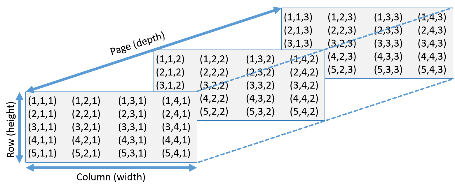![](http://www.socr.umich.edu/people/dinov/2017/Spring/DSPA_HS650/images/R_MatrixArrays_Diagram.png):	
#' 	
#' 	
ar<-array(1:24, dim=c(3, 4, 2))	
ar	
ar[2, 3, 1]	
ar[2, ,1]	
#' 	
#' 	
#' * In General, multi-dimensional arrays are called "tensors" (of order=number of dimensions).	
#' 	
#' Other useful functions are:	
#' 	
#' * `matrix(x, nrow=, ncol=)`: creates matrix elements of `nrow` rows and `ncol` columns.	
#' * `factor(x, levels=)`: encodes a vector `x` as a factor. 	
#' * `gl(n, k, length=n*k, labels=1:n)`: generate levels (factors) by specifying the pattern of their levels.	
#' *k* is the number of levels, and *n* is the number of replications.	
#' * `expand.grid()`: a data frame from all combinations of the supplied vectors or factors.	
#' * `rbind()` combine arguments by rows for matrices, data frames, and others	
#' * `cbind()` combine arguments by columns for matrices, data frames, and others	
#' 	
#' 	
#' # Input/Output(I/O)	
#' 	
#' The first pair of functions we will talk about are `load()`, which helps us reload datasets written with the `save()` function.	
#' 	
#' Let's create some data first.	
#' 	
x <- seq(1, 10, by=0.5)	
y <- list(a = 1, b = TRUE, c = "oops")	
save(x, y, file="xy.RData")	
load("xy.RData")	
#' 	
#' 	
#' `data(x)` loads specified data sets `library(x)` load add-on packages.	
#' 	
data("iris")	
summary(iris)	
#' 	
#' 	
#' **read.table(file)** reads a file in table format and creates a  data frame from it. The default separator `sep=""` is any whitespace. Use `header=TRUE` to read the first line as a header of column names. Use `as.is=TRUE` to prevent character vectors from being converted to factors. Use `comment.char=""` to prevent `"#"` from being interpreted as a comment. Use `skip=n` to skip `n` lines before reading data.  See the help for options on row naming, NA treatment, and others.	
#' 	
#' Let's use `read.table()` to read a text file in our class file.	
#' 	
data.txt<-read.table("https://umich.instructure.com/files/1628628/download?download_frd=1", header=T, as.is = T) # 01a_data.txt	
summary(data.txt)	
#' 	
#' 	
#' A note of caution; if you post data on a Cloud web service like Instructure/Canvas or GoogleDrive/GDrive that you want to process externally, e.g., via `R`, the direct URL reference to the raw file will be different from the URL of the pointer to the file that can be rendered in the browser window. For instance,	
#' 	
#'  - This [GDrive TXT file, *1Zpw3HSe-8HTDsOnR-n64KoMRWYpeBBek* (01a_data.txt)](https://drive.google.com/open?id=1Zpw3HSe-8HTDsOnR-n64KoMRWYpeBBek),	
#'  - [Can be downloaded and ingested in R via this separate URL](https://drive.google.com/uc?export=download&id=1Zpw3HSe-8HTDsOnR-n64KoMRWYpeBBek).	
#'  - While the file reference is unchanged (*1Zpw3HSe-8HTDsOnR-n64KoMRWYpeBBek*), note the change of syntax from viewing the file in the browser, **open?id=**, to auto-downloading the file for `R` processing, **uc?export=download&id=**.	
#' 	
#' 	
dataGDrive.txt<-read.table("https://drive.google.com/uc?export=download&id=1Zpw3HSe-8HTDsOnR-n64KoMRWYpeBBek", header=T, as.is = T) # 01a_data.txt	
summary(dataGDrive.txt)	
#' 	
#' 	
#' **read.csv("filename", header=TRUE)** is identical to `read.table()` but with defaults set for reading comma-delimited files.	
#' 	
data.csv<-read.csv("https://umich.instructure.com/files/1628650/download?download_frd=1", header = T)  # 01_hdp.csv	
summary(data.csv)	
#' 	
#' 	
#' **read.delim("filename", header=TRUE)** is very similar to the first two. However, it has defaults set for reading tab-delimited files.	
#' 	
#' Also we have `read.fwf(file, widths, header=FALSE, sep="\t", as.is=FALSE)` to read a table of fixed width formatted data into a data frame.	
#' 	
#' **match(x, y)** returns a vector of the positions of (first) matches of its first argument in its second. For a specific element in `x` if no elements matches it in `y` then the output for that elements would be `NA`.	
#' 	
match(c(1, 2, 4, 5), c(1, 4, 4, 5, 6, 7))	
#' 	
#' 	
#' **save.image(file)** saves all objects in the current work space.	
#' 	
#' **write.table(x, file="", row.names=TRUE, col.names=TRUE, sep="")** prints x after converting to a data frame and stores it into a specified file. If `quote` is TRUE, character or factor columns are surrounded by quotes ("). `sep` is the field separator. `eol` is the end-of-line separator. `na` is the string for missing values. Use `col.names=NA` to add a blank column header to get the column headers aligned correctly for spreadsheet input.	
#' 	
#' Most of the I/O functions have a file argument. This can often be a character string naming a file or a connection. `file=""` means the standard input or output. Connections can include files, pipes, zipped files, and R variables.	
#' 	
#' On windows, the file connection can also be used with `description = "clipboard"`. To read a table copied from Excel, use `x <- read.delim("clipboard")`	
#' 	
#' To write a table to the clipboard for Excel, use `write.table(x, "clipboard", sep="\t", col.names=NA)`	
#' 	
#' For database interaction, see packages RODBC, DBI, RMySQL, RPgSQL, and ROracle, as well as packages XML, hdf5, netCDF for reading other file formats. We will talk about some of them in later chapters.	
#' 	
#' *Note*, an alternative library called `rio` handles import/export of multiple data types with simple syntax.	
#' 	
#' # Slicing and extracting data		
#' 	
#' The following table can help us to understand how to index vectors.	
#' 	
#' Expression     |Explanation	
#' -------------- |-----------	
#' `x[n]`	       |nth element	
#' `x[-n]`	|all but the nth element	
#' `x[1:n]`|	first n elements	
#' `x[-(1:n)]`	|elements from n+1 to the end	
#' `x[c(1, 4, 2)]`|	specific elements	
#' `x["name"]`	 |element named "name"	
#' `x[x > 3]`	|all elements greater than 3	
#' `x[x > 3 & x < 5]`|	all elements between 3 and 5	
#' `x[x %in% c("a", "and", "the")]`| elements in the given set	
#' 	
#' Indexing lists are similar to indexing vectors but some of the symbols are different.	
#' 	
#' Expression     |Explanation	
#' -------------- |-----------	
#' `x[n]`	|list with n elements 	
#' `x[[n]]`|	nth element of the list	
#' `x[["name"]]`| element of the list named "name" 		
#' 	
#' Indexing for matrices is a higher dimensional version of indexing vectors.	
#' 	
#' Expression     |Explanation	
#' -------------- |-----------	
#' `x[i, j]`|	element at row i, column j 	
#' `x[i, ]` |	row i	
#' `x[, j]`	|column j 	
#' `x[, c(1, 3)]`| columns 1 and 3 	
#' `x["name", ]`| row named "name"	
#' 	
#' # Variable conversion		
#' 	
#' The following functions can be used to convert data types:	
#' 	
#' `as.array(x)`, `as.data.frame(x)`, `as.numeric(x)`, `as.logical(x)`, `as.complex(x)`, `as.character(x)`, ...	
#' 	
#' Typing `methods(as)` in the console will generate a complete list for variable conversion functions. 	
#' 	
#' # Variable information		
#' 	
#' The following functions will test if the each data element is a specific type:	
#' 	
#' `is.na(x)`, `is.null(x)`, `is.array(x)`, `is.data.frame(x)`, `is.numeric(x)`, `is.complex(x)`, `is.character(x)`, ...	
#' 	
#' For a complete list, type `methods(is)` in R console. The output for these functions are a bunch of `TRUE` or `FALSE` logical statements. One statement for one element in the dataset.	
#' 	
#' **length(x)** gives us the number of elements in `x`.	
#' 	
x<-c(1, 3, 10, 23, 1, 3)	
length(x)	
#' 	
#' 	
#' **dim(x)** retrieves or sets the dimension of an object.	
#' 	
x<-1:12	
dim(x)<-c(3, 4)	
x	
#' 	
#' 	
#' **dimnames(x)** retrieves or sets the dimension names of an object. For higher dimensional objects like matrix or arrays we can combine `dimnames()` with list.	
#' 	
dimnames(x)<-list(c("R1", "R2", "R3"), c("C1", "C2", "C3", "C4"))	
x	
#' 	
#' 	
#' **nrow(x)** number of rows; ncol(x) number of columns	
#' 	
nrow(x)	
ncol(x)	
#' 	
#' 	
#' **class(x)** get or set the class of x. Note that we can use `unclass(x)` to remove the class attribute of x. 	
#' 	
class(x)	
class(x)<-"myclass"	
x<-unclass(x)	
x	
#' 	
#' 	
#' **attr(x, which)** get or set the attribute `which` of x.	
#' 	
attr(x, "class")	
attr(x, "dim")<-c(2, 6)	
x	
#' 	
#' From the above commands we know that when we unclass `x`, its class would be `NULL`.	
#' 	
#' **attributes(obj)** get or set the list of attributes of object.	
#' 	
attributes(x) <- list(mycomment = "really special", dim = 3:4, 	
   dimnames = list(LETTERS[1:3], letters[1:4]), names = paste(1:12))	
x	
#' 	
#' 	
#' # Data selection and manipulation	
#' 	
#' In this section, we will introduce some data manipulation functions. In addition, tools from `dplyr` provide easy dataset manipulation routines.	
#' 	
#' **which.max(x)** returns the index of the greatest element of x. **which.min(x)** returns the index of the smallest element of x. **rev(x)** reverses the elements of x. Let's see these three functions first.	
#' 	
#' 	
x<-c(1, 5, 2, 1, 10, 40, 3)	
which.max(x)	
which.min(x)	
rev(x)	
#' 	
#' 	
#' **sort(x)** sorts the elements of x in increasing order. To sort in decreasing order we can use `rev(sort(x))`.	
#' 	
sort(x)	
rev(sort(x))	
#' 	
#' 	
#' **cut(x, breaks)** divides x into intervals with same length (sometimes factors). `breaks` is the number of cut intervals or a vector of cut points. `cut` divides the range of x into intervals coding the values in x according to the intervals they fall into.	
#' 	
x	
cut(x, 3)	
cut(x, c(0, 5, 20, 30))	
#' 	
#' 	
#' **which(x == a)** returns a vector of the indices of `x` if the comparison operation is true (TRUE). For example it returns the value `i`, if `x[i]== a` is true. Thus, the argument of this function (like `x==a`) must be a variable of mode logical.	
#' 	
x	
which(x==2)	
#' 	
#' 	
#' **na.omit(x)** suppresses the observations with missing data (`NA`). It suppresses the corresponding line if x is a matrix or a data frame. **na.fail(x)** returns an error message if x contains at least one `NA`.	
#' 	
df<-data.frame(a=1:5, b=c(1, 3, NA, 9, 8))	
df	
na.omit(df)	
#' 	
#' 	
#' **unique(x)** If x is a vector or a data frame, it returns a similar object but with the duplicate elements suppressed.	
#' 	
df1<-data.frame(a=c(1, 1, 7, 6, 8), b=c(1, 1, NA, 9, 8))	
df1	
unique(df1)	
#' 	
#'  	
#' **table(x)** returns a table with the different values of x and their frequencies (typically for integers or factors). Also check `prop.table()`.	
#' 	
#' 	
v<-c(1, 2, 4, 2, 2, 5, 6, 4, 7, 8, 8)	
table(v)	
#' 	
#' 	
#' **subset(x, ...)** returns a selection of x with respect to criteria `...` (typically `...` are comparisons like `x$V1 < 10`). If x is a data frame, the option `select=` gives the variables to be kept or dropped using a minus sign.	
#' 	
sub<-subset(df1, df1$a>5)	
sub	
sub<-subset(df1, select=-a)	
sub	
#' 	
#' 	
#' **sample(x, size)** resample randomly and without replacement size elements in the vector `x`, the option `replace = TRUE` allows to resample with replacement.	
#' 	
df1<-data.frame(a=c(1, 1, 7, 6, 8), b=c(1, 1, NA, 9, 8))	
sample(df1$a, 20, replace = T)	
#' 	
#' 	
#' **prop.table(x, margin=)** table entries as fraction of marginal table.	
#' 	
prop.table(table(v))	
#' 	
#' 	
#' # Mathematics, Statistics, and Optimization	
#' 	
#' ## Math Functions		
#' 	
#' Basic math functions like `sin`, `cos`, `tan`, `asin`, `acos`, `atan`, `atan2`, `log`, `log10`, `exp` and "set" functions `union(x, y)`, `intersect(x, y)`, `setdiff(x, y)`, `setequal(x, y)`, `is.element(el, set)` are available in R.	
#' 	
#' `lsf.str("package:base")` displays all base function built in a specific R package (like `base`).	
#' 	
#' Also we have the following table of functions that you might need when use R for calculations.	
#' 	
#' Expression           |Explanation	
#' ---------------------|-------------------------------------------------------------	
#' `choose(n, k)`| computes the combinations of k events among n repetitions. Mathematically it equals to  $\frac{n!}{[(n-k)!k!]}$	
#' `max(x)`| maximum of the elements of x	
#' `min(x)`| minimum of the elements of x 	
#' `range(x)`| minimum and maximum of the elements of x 	
#' `sum(x)`| sum of the elements of x	
#' `diff(x)`| lagged and iterated differences of vector x	
#' `prod(x)`| product of the elements of x 	
#' `mean(x)`| mean of the elements of x 	
#' `median(x)`| median of the elements of x	
#' `quantile(x, probs=)`| sample quantiles corresponding to the given probabilities (defaults to 0, .25, .5, .75, 1)	
#' `weighted.mean(x, w)`| mean of x with weights w	
#' `rank(x)`| ranks of the elements of x	
#' `var(x)` or `cov(x)`| variance of the elements of x (calculated on n>1). If x is a matrix or a data frame, the variance-covariance matrix is calculated	
#' `sd(x)`| standard deviation of x	
#' `cor(x)`| correlation matrix of x if it is a matrix or a data frame (1 if x is a vector)	
#' `var(x, y)` or `cov(x, y)`| covariance between x and y, or between the columns of x and those of y if they are matrices or data frames	
#' `cor(x, y)`| linear correlation between x and y, or correlation matrix if they are matrices or data frames	
#' `round(x, n)`| rounds the elements of x to n decimals	
#' `log(x, base)`| computes the logarithm of x with base base	
#' `scale(x)`| if x is a matrix, centers and reduces the data. Without centering use the option `center=FALSE`. Without scaling use `scale=FALSE` (by default center=TRUE, scale=TRUE)	
#' `pmin(x, y, ...)`| a vector which ith element is the minimum of x[i], y[i], . . .	
#' `pmax(x, y, ...)`| a vector which ith element is the maximum of x[i], y[i], . . .	
#' `cumsum(x)`| a vector which ith element is the sum from x[1] to x[i]	
#' `cumprod(x)`| id. for the product 	
#' `cummin(x)`| id. for the minimum 	
#' `cummax(x)`| id. for the maximum	
#' `Re(x)`|real part of a complex number	
#' `Im(x)`| imaginary part of a complex number	
#' `Mod(x)`| modulus. `abs(x)` is the same	
#' `Arg(x)`| angle in radians of the complex number	
#' `Conj(x)`| complex conjugate	
#' `convolve(x, y)`| compute the several kinds of convolutions of two sequences	
#' `fft(x)`| Fast Fourier Transform of an array	
#' `mvfft(x)`| FFT of each column of a matrix	
#' `filter(x, filter)`| applies linear filtering to a univariate time series or to each series separately of a multivariate time series	
#' 	
#' Note: many math functions have a logical parameter `na.rm=TRUE` to specify missing data (`NA`) removal.	
#' 	
#' ## Matrix Operations		
#' 	
#' The following table summarizes basic operation functions. We will discuss this topic in detail in [Chapter 4](https://www.socr.umich.edu/people/dinov/courses/DSPA_notes/04_LinearAlgebraMatrixComputing.html).	
#' 	
#' Expression    |Explanation	
#' --------------|-------------------------------------------------------------------	
#' `t(x)`| transpose	
#' `diag(x)`| diagonal	
#' `%*%`| matrix multiplication	
#' `solve(a, b)`| solves `a %*% x = b` for x	
#' `solve(a)`| matrix inverse of a	
#' `rowsum(x)`| sum of rows for a matrix-like object. `rowSums(x)` is a faster version	
#' `colsum(x)`, `colSums(x)`| id. for columns 	
#' `rowMeans(x)`| fast version of row means 	
#' `colMeans(x)`| id. for columns	
#' 	
#' 	
mat1 <- cbind(c(1, -1/5), c(-1/3, 1))	
mat1.inv <- solve(mat1)	
	
mat1.identity <- mat1.inv %*% mat1	
mat1.identity	
b <- c(1, 2)	
x <- solve (mat1, b)	
x	
#' 	
#' 	
#' ## Optimization and model fitting		
#' 	
#'  **optim(par, fn, method = c("Nelder-Mead", "BFGS", "CG", "L-BFGS-B", "SANN"))** general-purpose optimization; `par` is initial values, `fn` is function to optimize (normally minimize).	
#' 	
#'  **nlm(f, p)** minimize function fusing a Newton-type algorithm with starting values p.	
#' 	
#'  **lm(formula)** fit linear models; `formula` is typically of the form `response ~ termA + termB + ...`; use `I(x*y) + I(x^2)` for terms made of nonlinear components.	
#' 	
#'  **glm(formula, family=)** fit generalized linear models, specified by giving a symbolic description of the linear predictor and a description of the error distribution; `family` is a description of the error distribution and link function to be used in the model; see `?family`.	
#' 	
#'  **nls(formula)** nonlinear least-squares estimates of the nonlinear model parameters.	
#' 	
#'  **approx(x, y=)** linearly interpolate given data points; x can be an xy plotting structure.	
#' 	
#'  **spline(x, y=)** cubic spline interpolation.	
#' 	
#'  **loess(formula)** (locally weighted scatterplot smoothing) fit a polynomial surface using local fitting.	
#' 	
#' Many of the formula-based modeling functions have several common arguments:	
#' 	
#' `data=` the data frame for the formula variables, `subset=` a subset of variables used in the fit, `na.action=` action for missing values: `"na.fail"`, `"na.omit"`, or a function. 	
#' 	
#' The following generics often apply to model fitting functions:	
#' 	
#' `predict(fit, ...)` predictions from fit based on input data.	
#' 	
#' `df.residual(fit)` returns the number of residual degrees of freedom. 	
#' 	
#' `coef(fit)` returns  the  estimated  coefficients  (sometimes  with  their standard-errors). 	
#' 	
#' `residuals(fit)` returns the residuals.	
#' 	
#' `deviance(fit)` returns the deviance.	
#' 	
#' `fitted(fit)` returns the fitted values.	
#' 	
#' `logLik(fit)` computes the logarithm of the likelihood and the number of parameters.	
#' 	
#' `AIC(fit)` computes the Akaike information criterion (AIC).	
#' 	
#' ## Statistics		
#' 	
#' **aov(formula)** analysis of variance model.	
#' 	
#' **anova(fit, ...)** analysis of variance (or deviance) tables for one or more fitted model objects.	
#' 	
#' **density(x)** kernel density estimates of x.	
#' 	
#' Other functions include: `binom.test()`, 	`pairwise.t.test()`, 	`power.t.test()`, `prop.test()`, `t.test()`, ... use `help.search("test")` to see details.	
#' 	
#' ## Distributions	
#' 	
#' Random sample generation from different distributions. Remember to include `set.seed()` if you want to get reproducibility during exercises.	
#' 	
#' Expression                       |Explanation	
#' ---------------------------------|-----------	
#' `rnorm(n, mean=0, sd=1)`| Gaussian (normal)	
#' `rexp(n, rate=1)`| exponential	
#' `rgamma(n, shape, scale=1)`| gamma	
#' `rpois(n, lambda)`| Poisson	
#' `rweibull(n, shape, scale=1)`| Weibull 	
#' `rcauchy(n, location=0, scale=1)`| Cauchy 	
#' `rbeta(n, shape1, shape2)`| beta	
#' `rt(n, df)`| Student's (t)	
#' `rf(n, df1, df2)`| Fisher's (F) (df1, df2)	
#' `rchisq(n, df)`| Pearson rbinom(n, size, prob) binomial 	
#' `rgeom(n, prob)`| geometric	
#' `rhyper(nn, m, n, k)`| hypergeometric 	
#' `rlogis(n, location=0, scale=1)`| logistic	
#' `rlnorm(n, meanlog=0, sdlog=1)`| lognormal 	
#' `rnbinom(n, size, prob)`| negative binomial 	
#' `runif(n, min=0, max=1)`| uniform	
#' `rwilcox(nn, m, n)`, `rsignrank(nn, n)`| Wilcoxon's statistics	
#' 	
#' Also all these functions can be used by replacing the letter `r` with `d`, `p` or `q` to get, respectively, the probability density (`dfunc(x, ...)`), the cumulative probability density (`pfunc(x, ...)`), and the value of quantile (`qfunc(p, ...)`, with $0 < p < 1$).	
#' 	
#' 	
#' # Advanced Data Processing		
#' 	
#' In this section, we will introduce some fancy functions that can save time remarkably.	
#' 	
#' **apply(X, INDEX, FUN=)** a vector or array or list of values obtained by applying a function `FUN` to margins (`INDEX=1` means row, `INDEX=2` means column) of X.	
#' 	
df1	
apply(df1, 2, mean, na.rm=T)	
#' 	
#' Note that we can add options for the `FUN` after the function.	
#' 	
#' **lapply(X, FUN)** apply `FUN` to each member of the list X. If X is a data frame then it will apply the `FUN` to each column and return a list. 	
#' 	
lapply(df1, mean, na.rm=T)	
lapply(list(a=c(1, 23, 5, 6, 1), b=c(9, 90, 999)), median)	
#' 	
#' 	
#' **tapply(X, INDEX, FUN=)** apply `FUN` to each cell of a ragged array given by X with indexes equals to `INDEX`. Note that X is an atomic object, typically a vector	
#' 	
v	
fac <- factor(rep(1:3, length = 11), levels = 1:3)	
table(fac)	
tapply(v, fac, sum)	
#' 	
#' 	
#' **by(data, INDEX, FUN)** apply `FUN` to data frame data subsetted by INDEX.	
#' 	
by(df1, df1[, 1], sum)	
#' 	
#' The above line of code apply the `sum` function using column 1(`a`) as an index.	
#' 	
#' **merge(a, b)** merge two data frames by common columns or row names. We can use option `by=` to specify the index column.	
#' 	
df2<-data.frame(a=c(1, 1, 7, 6, 8), c=1:5)	
df2	
df3<-merge(df1, df2, by="a")	
df3	
#' 	
#' 	
#' **xtabs(a ~ b, data=x)** a contingency table from cross-classifying factors.	
#' 	
#' 	
DF <- as.data.frame(UCBAdmissions)	
##  'DF' is a data frame with a grid of the factors and the counts	
## in variable 'Freq'.	
DF	
## Nice for taking margins ...	
xtabs(Freq ~ Gender + Admit, DF)	
## And for testing independence ...	
summary(xtabs(Freq ~ ., DF))	
#' 	
#' 	
#' **aggregate(x, by, FUN)** splits the data frame x into subsets, computes summary statistics for each, and returns the result in a convenient form. `by` is a list of grouping elements, each has the same length as the variables in x.	
#' 	
#' 	
list(rep(1:3, length=7))	
aggregate(df3, by=list(rep(1:3, length=7)), sum)	
#' 	
#' 	
#' The above code applied function `sum` to data frame `df3` according to the index created by `list(rep(1:3, length=7))`.	
#' 	
#' **stack(x, ...)** transform data available as separate columns in a data frame or list into a single column.	
#' and `unstack(x, ...)` is inverse of `stack()`.	
#' 	
stack(df3)	
unstack(stack(df3))	
#' 	
#' 	
#' **reshape(x, ...)** reshapes a data frame between "wide" format with repeated measurements in separate columns of the same record and "long" format with the repeated measurements in separate records. Use `direction="wide"` or `direction="long"`.	
#' 	
#' 	
df4 <- data.frame(school = rep(1:3, each = 4), class = rep(9:10, 6), 	
                  time = rep(c(1, 1, 2, 2), 3), score = rnorm(12))	
wide <- reshape(df4, idvar = c("school", "class"), direction = "wide")	
wide	
	
long <- reshape(wide, idvar = c("school", "class"), direction = "long")	
long	
#' 	
#' 	
#' <!---	
#' # See: http://stats.idre.ucla.edu/r/faq/how-can-i-reshape-my-data-in-r/	
#' 	
#' # wiki_url <- read_html("https://wiki.socr.umich.edu/index.php/SOCR_Data_PD_BiomedBigMetadata")	
#' #html_nodes(wiki_url, "#content")	
#' #pd_data <- html_table(html_nodes(wiki_url, "table")[[1]])	
#' #head(pd_data); summary(pd_data)	
#' long <- reshape(pd_data, 	
#'   varying = "Time", 	
#'   v.names = c("Time1", "Time2", "Time3", "Time4")  # colnames(pd_data)[-33],	
#'   times = "Time", 	
#'   direction = "long")	
#'   	
#' # arguments include 	
#' # (1) list of variable names that define the different times or metrics (varying), 	
#' # (2) the name we wish to give the variable containing these values in our long dataset (v.names), 	
#' # (3) the name we wish to give the variable describing the different times or metrics (timevar), 	
#' # (4) the values this variable will have (times), and 	
#' # (5) the end format for the data (direction)	
#' 	
#' wide <- reshape(pd_data, 	
#'   timevar = "Time",	
#'   idvar = colnames(pd_data)[-33],	
#'   direction = "wide")	
#'  	
#' # To reshape the PD dataset into wide format, we will use the reshape function. The arguments we provide include 	
#' ### (1) *direction* = "wide" 	
#' ### (2) *timevar*, we indicate the variable that will define the multiple measurements per subject. 	
#' ### (3) *idvar* list the variables that should do not vary within subject.	
#' --->	
#' 	
#' **Notes**	
#' 	
#' * The $x$ in this function has to be longitudinal data.	
#' * The call to `rnorm` used in reshape might generate different results for each call, unless `set.seed(1234)` is used to ensure reproducibility of random-number generation.	
#' 	
#' # Strings		
#' 	
#' The following functions are useful for handling strings in R.	
#' 	
#' **paste(...)** concatenate vectors after converting to character. It has a few options. `sep=` is the string to separate terms (a single space is the default). `collapse=` is an optional string to separate "collapsed" results.	
#' 	
a<-"today"	
b<-"is a good day"	
paste(a, b)	
paste(a, b, sep=", ")	
#' 	
#' 	
#' **substr(x, start, stop)** substrings in a character vector. It can also assign values (with the same length) to part of a string, as `substr(x, start, stop) <- value`.	
#' 	
#' 	
a<-"When the going gets tough, the tough get going!"	
substr(a, 10, 40)	
## [1] "going gets tough, the tough get"	
substr(a, 1, 9)<-"........."	
a	
#' 	
#' 	
#' Note that characters at `start` and `stop` indexes are inclusive in the output.	
#' 	
#' **strsplit(x, split)** split x according to the substring split. Use `fixed=TRUE` for non-regular expressions.	
#' 	
strsplit("a.b.c", ".", fixed = TRUE)	
#' 	
#' 	
#' **grep(pattern, x)** searches for matches to pattern within x. It will return a vector of the indices of the elements of x that yielded a match. Use regular expression for `pattern`(unless `fixed=TRUE`). See `?regex` for details.	
#' 	
#' 	
letters	
grep("[a-z]", letters)	
#' 	
#' 	
#' **gsub(pattern, replacement, x)** replacement of matches determined by regular expression matching. **sub()** is the same but only replaces the first occurrence.	
#' 	
a<-c("e", 0, "kj", 10, ";")	
gsub("[a-z]", "letters", a)	
sub("[a-z]", "letters", a)	
#' 	
#' 	
#' **tolower(x)** convert to lowercase. **toupper(x)** convert to uppercase.	
#' 	
#' **match(x, table)** a vector of the positions of first matches for the elements of x among `table`. `x %in% table` id. but returns a logical vector.	
#' 	
x<-c(1, 2, 10, 19, 29)	
match(x, c(1, 10))	
x %in% c(1, 10)	
#' 	
#' 	
#' **pmatch(x, table)** partial matches for the elements of x among table.	
#' 	
pmatch("m",   c("mean", "median", "mode")) # returns NA	
pmatch("med", c("mean", "median", "mode")) # returns 2	
#' 	
#' The first one returns `NA`, and dependent on the R-version possibly a warning, because all elements have the pattern `"m"`.	
#' 	
#' **nchar(x)** number of characters	
#' 	
#' **Dates and Times**	
#' 	
#' The class `Date` has dates without times. `POSIXct()` has dates and times, including time zones. Comparisons (e.g. >), `seq()`, and `difftime()` are useful. `?DateTimeClasses` gives more information. See also package `chron`.	
#' 	
#' `as.Date(s)` and `as.POSIXct(s)` convert to the respective class; `format(dt)` converts to a string representation. The default string format is `2001-02-21`. These accept a second argument to specify a format for conversion. Some common formats are:	
#' 	
#' Formats           | Explanations	
#' ------------------|---------------------------------------------------------------	
#' `%a, %A`| Abbreviated and full weekday name.	
#' `%b, %B`| Abbreviated and full month name.	
#' `%d` |Day of the month (01 ... 31).	
#' `%H`| Hours (00 ... 23).	
#' `%I`| Hours (01 ... 12).	
#' `%j`| Day of year (001 ... 366).	
#' `%m`| Month (01 ... 12).	
#' `%M`| Minute (00 ... 59).	
#' `%p`| AM/PM indicator.	
#' `%S`| Second as decimal number (00 ... 61).	
#' `%U`| Week (00 ... 53); the first Sunday as day 1 of week 1.	
#' `%w`| Weekday (0 ... 6, Sunday is 0).	
#' `%W`| Week (00 ... 53); the first Monday as day 1 of week 1.	
#' `%y`| Year without century (00 ... 99). Don't use.	
#' `%Y`| Year with century.	
#' `%z` (output only.)| Offset from Greenwich; -0800 is 8 hours west of.	
#' `%Z` (output only.)| Time zone as a character string (empty if not available).	
#' 	
#' Where leading zeros are shown they will be used on output but are optional on input. See `?strftime` for details.	
#' 	
#' # Plotting		
#' 	
#' This only an introduction for plotting functions in R. In [Chapter 2](https://www.socr.umich.edu/people/dinov/2017/Spring/DSPA_HS650/notes/03_DataVisualization.html), we will discuss visualization in more detail.	
#' 	
#'  **plot(x)** plot of the values of x (on the y-axis) ordered on the x-axis.	
#' 	
#'  **plot(x, y)** bivariate plot of x (on the x-axis) and y (on the y-axis).	
#' 	
#'  **hist(x)** histogram of the frequencies of x.	
#' 	
#'  **barplot(x)** histogram of the values of x. Use `horiz=FALSE` for horizontal bars.	
#' 	
#'  **dotchart(x)** if x is a data frame, plots a Cleveland dot plot (stacked plots line-by-line and column-by-column).	
#' 	
#'  **pie(x)** circular pie-chart.	
#' 	
#'  **boxplot(x)** 'box-and-whiskers' plot.	
#' 	
#'  **sunflowerplot(x, y)** id. than plot() but the points with similar coordinates are drawn as flowers which petal number represents the number of points.	
#' 	
#'  **stripplot(x)** plot  of  the  values  of  x on  a  line  (an  alternative  to `boxplot()` for small sample sizes).	
#' 	
#'  **coplot(x~y |  z)** bivariate plot of x and y for each value or interval of values of z.	
#' 	
#'  **interaction.plot (f1, f2, y)** if f1 and f2 are factors, plots the means of y (on the y-axis) with respect to the values of f1 (on the x-axis) and of f2 (different curves). The option `fun` allows to choose the summary statistic of y (by default `fun=mean`).	
#' 	
#'  **matplot(x, y)** bivariate plot of the first column of x vs. the first one of y, the second one of x vs. the second one of y, etc.	
#' 	
#'  **fourfoldplot(x)** visualizes, with quarters of circles, the association between two dichotomous variables for different populations (x must be an array with dim=c(2, 2, k), or a matrix with dim=c(2, 2) if k = 1)	
#' 	
#'  **assocplot(x)** Cohen's Friendly graph shows the deviations from independence of rows and columns in a two dimensional contingency table.	
#' 	
#'  **mosaicplot(x)** "mosaic"" graph of the residuals from a log-linear regression of a contingency table.	
#' 	
#'  **pairs(x)** if x is a matrix or a data frame, draws all possible bivariate plots between the columns of x.	
#' 	
#'  **plot.ts(x)** if x is an object of class "ts", plot of x with respect to time, x may be multivariate but the series must have the same frequency and dates. Detailed examples are in **Chapter 17: Big Longitudinal Data Analysis**.	
#' 	
#'  **ts.plot(x)** id. but if x is multivariate the series may have different dates and must have the same frequency.	
#' 	
#'  **qqnorm(x)** quantiles of x with respect to the values expected under a normal law.	
#' 	
#'  **qqplot(x, y)** quantiles of y with respect to the quantiles of x.	
#' 	
#'  **contour(x, y, z)** contour plot (data are interpolated to draw the curves), x and y must be vectors and z must be a matrix so that `dim(z)=c(length(x), length(y))` (x and y may be omitted).	
#' 	
#'  **filled.contour(x, y, z)** areas between the contours are colored, and a legend of the colors is drawn as well.	
#' 	
#'  **image(x, y, z)** plotting actual data with colors.	
#' 	
#'  **persp(x, y, z)** plotting actual data in perspective view.	
#' 	
#'  **stars(x)** if x is a matrix or a data frame, draws a graph with segments or a star where each row of x is represented by a star and the columns are the lengths of the segments.	
#' 	
#'  **symbols(x, y, ...)** draws, at the coordinates given by x and y, symbols (circles, squares, rectangles, stars, thermometers or "boxplots"") which sizes, colors... are specified by supplementary arguments.	
#' 	
#'  **termplot(mod.obj)** plot of the (partial) effects of a regression model (`mod.obj`).	
#' 	
#' The following parameters are common to many plotting functions: 	
#' 	
#' Parameters  | Explanations	
#' ------------|--------------------------------------------------------------	
#' `add=FALSE`| if TRUE superposes the plot on the previous one (if it exists) 	
#' `axes=TRUE`| if FALSE does not draw the axes and the box	
#' `type="p"`| specifies the type of plot, "p": points, "l": lines, "b": points connected by lines, "o": id. But the lines are over the points, "h": vertical lines, "s": steps, the data are represented by the top of the vertical lines, "S": id. However, the data are represented at the bottom of the vertical lines	
#' `xlim=, ylim=`| specifies the lower and upper limits of the axes, for example with `xlim=c(1, 10)` or `xlim=range(x)`	
#' `xlab=, ylab=`| annotates the axes, must be variables of mode character 	
#' `main=`| main title, must be a variable of mode character	
#' `sub=`| subtitle (written in a smaller font)	
#' 	
#' ## QQ Normal probability plot 	
#' 	
#' Let's look at one simple example - quantile-quantile probability plot. Suppose $X\sim N(0,1)$ and $Y\sim Cauchy$ represent the observed/raw and simulated/generated data for one feature (variable) in the data.	
#' 	
#' 	
X_norm1 <- rnorm(1000)	
X_norm2 <- rnorm(1000, m=-75, sd=3.7)	
X_Cauchy <- rcauchy(1000)	
	
# compare X to StdNormal distribution	
# 	qqnorm(X, 	
#          		main="Normal Q-Q Plot of the data", 	
#          		xlab="Theoretical Quantiles of the Normal", 	
#          		ylab="Sample Quantiles of the X (Normal) Data")	
# 	qqline(X)	
# 	qqplot(X, Y)	
fit_norm_norm = lm(X_norm2 ~ X_norm1)	
fit_norm_cauchy = lm(X_Cauchy ~ X_norm1)	
	
# Get model fitted values	
Fitted.Values.norm_norm <-  fitted(fit_norm_norm)	
Fitted.Values.norm_cauchy <-  fitted(fit_norm_cauchy)	
  	
# Extract model residuals	
Residuals.norm_norm <-  resid(fit_norm_norm)	
Residuals.norm_cauchy <-  resid(fit_norm_cauchy)	
	
# Compute the model standardized residuals from lm() object	
Std.Res.norm_norm <- MASS::stdres(fit_norm_norm)  	
Std.Res.norm_cauchy <- MASS::stdres(fit_norm_cauchy)  	
  	
# Extract the theoretical (Normal) quantiles	
Theoretical.Quantiles.norm_norm <- qqnorm(Residuals.norm_norm, plot.it = F)$x	
Theoretical.Quantiles.norm_cauchy <- qqnorm(Residuals.norm_cauchy, plot.it = F)$x	
  	
qq.df.norm_norm <- data.frame(Std.Res.norm_norm, Theoretical.Quantiles.norm_norm)	
qq.df.norm_cauchy <- data.frame(Std.Res.norm_cauchy, Theoretical.Quantiles.norm_cauchy)	
	
qq.df.norm_norm %>% 	
  plot_ly(x = ~Theoretical.Quantiles.norm_norm) %>% 	
    add_markers(y = ~Std.Res.norm_norm, name="Normal(0,1) vs. Normal(-75, 3.7) Data") %>%	
    add_lines(x = ~Theoretical.Quantiles.norm_norm, y = ~Theoretical.Quantiles.norm_norm, 	
              mode = "line", name = "Theoretical Normal", line = list(width = 2)) %>% 	
    layout(title = "Q-Q Normal Plot", legend = list(orientation = 'h'))	
	
# Normal vs. Cauchy	
qq.df.norm_cauchy %>% 	
  plot_ly(x = ~Theoretical.Quantiles.norm_cauchy) %>% 	
    add_markers(y = ~Std.Res.norm_cauchy, name="Normal(0,1) vs. Cauchy Data") %>%	
    add_lines(x = ~Theoretical.Quantiles.norm_norm, y = ~Theoretical.Quantiles.norm_norm, 	
              mode = "line", name = "Theoretical Normal", line = list(width = 2)) %>% 	
    layout(title = "Normal vs. Cauchy Q-Q Plot", legend = list(orientation = 'h'))	
	
# Q-Q plot data (X) vs. simulation(Y)	
# 	
# myQQ <- function(x, y, ...) {	
#   #rang <- range(x, y, na.rm=T)	
#   rang <- range(-4, 4, na.rm=T)	
#   qqplot(x, y, xlim=rang, ylim=rang)	
# }	
# 	
# myQQ(X, Y) # where the Y is the newly simulated data for X	
# qqline(X)	
#' 	
#' 	
#' ## Subsampling	
#' 	
#' 	
x <- matrix(rnorm(100), ncol = 5)	
y <- c(1, seq(19))	
	
z <- cbind(x, y)	
	
z.df <- data.frame(z)	
z.df	
	
names(z.df)	
# subsetting rows	
z.sub <- subset(z.df, y > 2 & (y<10 | V1>0))	
z.sub	
	
z.sub1 <- z.df[z.df$y == 1, ]	
z.sub1	
z.sub2 <- z.df[z.df$y %in% c(1, 4), ]	
z.sub2	
	
# subsetting columns	
z.sub6 <- z.df[, 1:2]	
z.sub6	
#' 	
#' 	
#' ## Low-level plotting commands	
#' 	
#'  **points(x, y)** adds points (the option `type=` can be used)	
#' 	
#'  **lines(x, y)** id. but with lines	
#' 	
#'  **text(x, y, labels, ...)** adds text given by labels at coordinates (x, y). Typical use: `plot(x, y, type="n"); text(x, y, names)`	
#' 	
#'  **mtext(text, side=3, line=0, ...)** adds text given by text in the margin specified by side (see `axis()` below); line specifies the line from the plotting area.	
#' 	
#'  **segments(x0, y0, x1, y1)** draws lines from points `(x0, y0)` to points `(x1, y1)`	
#' 	
#'  **arrows(x0, y0, x1, y1, angle= 30, code=2)** id. With arrows at points `(x0, y0)`, if `code=2`. The arrow is at point `(x1, y1)`, if `code=1`. Arrows are at both if `code=3`. Angle controls the angle from the shaft of the arrow to the edge of the arrow head.	
#' 	
#'  **abline(a, b)** draws a line of slope `b` and intercept `a`.	
#' 	
#'  **abline(h=y)** draws a horizontal line at ordinate y.	
#' 	
#'  **abline(v=x)** draws a vertical line at abscissa x. 	
#' 	
#'  **abline(lm.obj)** draws the regression line given by `lm.obj`.  abline(h=0, col=2) #color (col) is often used	
#' 	
#'  **rect(x1, y1, x2, y2)** draws a rectangle which left, right, bottom, and top limits are x1, x2, y1, and y2, respectively.	
#' 	
#'  **polygon(x, y)** draws a polygon linking the points with coordinates given by x and y.	
#' 	
#'  **legend(x, y, legend)** adds the legend at the point `(x, y)` with the symbols given by `legend`.	
#' 	
#'  **title()** adds a title and optionally a subtitle.	
#' 	
#'  **axis(side, vect)** adds an axis at the bottom (`side=1`), on the left (`side=2`), at the top (`side=3`), or on the right (`side=4`); `vect` (optional) gives the abscissa (or ordinates) where tick-marks are drawn.	
#' 	
#'  **rug(x)** draws the data x on the x-axis as small vertical lines.	
#' 	
#'  **locator(n, type="n", ...)** returns the coordinates `(x, y)` after the user has clicked n times on the plot with the mouse; also draws symbols (`type="p"`) or lines (`type="l"`) with respect to optional graphic parameters (...); by default nothing is drawn (`type="n"`).	
#' 	
#' ## General graphics parameters	
#' 	
#' These can be set globally with **par(...)**. Many can be passed as parameters to plotting commands.	
#' 	
#'  **adj** controls text justification (`adj=0` left-justified, `adj=0.5` centered, `adj=1` right-justified).	
#' 	
#'  **bg** specifies the color of the background (ex. : `bg="red"`, `bg="blue"`, ...the list of the 657 available colors is displayed with `colors()`).	
#' 	
#'  **bty** controls the type of box drawn around the plot. Allowed values are: "o", "l", "7", "c", "u" ou "]" (the box looks like the corresponding character). If `bty="n"` the box is not drawn.	
#' 	
#'  **cex** a value controlling the size of texts and symbols with respect to the default. The following parameters have the same control for numbers on the axes-`cex.axis`, the axis labels-`cex.lab`, the title-`cex.main`, and the subtitle-`cex.sub`.	
#' 	
#'  **col** controls the color of symbols and lines. Use color names: "red", "blue" see `colors()` or as "#RRGGBB"; see `rgb()`, `hsv()`, `gray()`, and `rainbow()`; as for cex there are: `col.axis`, `col.lab`, `col.main`, `col.sub`.	
#' 	
#'  **font** an integer which controls the style of text (1: normal, 2: italics, 3: bold, 4: bold italics); as for cex there are: `font.axis`, `font.lab`, `font.main`, `font.sub`.	
#' 	
#'  **las** an integer which controls the orientation of the axis labels (0: parallel to the axes, 1: horizontal, 2: perpendicular to the axes, 3: vertical).	
#' 	
#'  **lty** controls the type of lines, can be an integer or string (1: "solid", 2: "dashed",  3: "dotted",  4: "dotdash",  5: "longdash",  6: "twodash", or a string of up to eight characters (between "0" and "9") which specifies alternatively the length, in points or pixels, of the drawn elements and the blanks, for example `lty="44"` will have the same effect than `lty=2`.	
#' 	
#'  **lwd** a numeric which controls the width of lines, default=1.	
#' 	
#'  **mar** a vector of 4 numeric values which control the space between the axes and the border of the graph of the form `c(bottom, left, top, right)`, the default values are `c(5.1, 4.1, 4.1, 2.1)`.	
#' 	
#'  **mfcol** a vector of the form `c(nr, nc)` which partitions the graphic window as a matrix of nr lines and nc columns, the plots are then drawn in columns.	
#' 	
#'  **mfrow** id. but the plots are drawn by row.	
#' 	
#'  **pch** controls the type of symbol, either an integer between 1 and 25, or any single character within "".	
#'  	
#'  **ts.plot(x)** id. but if x is multivariate the series may have different dates by x and y.	
#'  	
#'  **ps** an integer which controls the size in points of texts and symbols.	
#' 	
#'  **pty** a character, which specifies the type of the plotting region, "s": square, "m": maximal.	
#' 	
#'  **tck** a value which specifies the length of tick-marks on the axes as a fraction of the smallest of the width or height of the plot; if `tck=1` a grid is drawn.	
#' 	
#'  **tcl** a value which specifies the length of tick-marks on the axes as a fraction of the height of a line of text (by default `tcl=-0.5`).	
#' 	
#'  **xaxt** if `xaxt="n"` the x-axis is set but not drawn (useful in conjunction with `axis(side=1, ...)`).	
#' 	
#'  **yaxt** if `yaxt="n"` the y-axis is set but not drawn (useful in conjunction with `axis(side=2, ...)`).	
#' 	
#'  ***Lattice (Trellis) graphics***	
#' 	
#' Expression         | Explanation	
#' -------------------|--------------------------------	
#' **xyplot(y~x)**    | bivariate plots (with many functionalities). 	
#' **barchart(y~x)**  | histogram of the values of y with respect to those of x.	
#' **dotplot(y~x)**   | Cleveland dot plot (stacked plots line-by-line and column-by-column)	
#' **densityplot(~x)** |  density functions plot 	
#' **histogram(~x)** | histogram of the frequencies of x 	
#' **bwplot(y~x)**   | "box-and-whiskers" plot	
#' **qqmath(~x)**    | quantiles of x with respect to the values expected under a theoretical distribution	
#' **stripplot(y~x)**  | single dimension plot, x must be numeric, y may be a factor	
#' **qq(y~x)**         | quantiles to compare two distributions, x must be numeric, y may be numeric, character, or factor but must have two "levels"	
#' **splom(~x)**      | matrix of bivariate plots	
#' **parallel(~x)**   | parallel coordinates plot	
#' levelplot($z\sim x*y\|g1*g2$)   | colored plot of the values of z at the coordinates given by x and y (x, y and z are all of the same length)	
#' wireframe($z\sim x*y\|g1*g2$)   | 3d surface plot	
#' cloud($z\sim x*y\|g1*g2$)   | 3d scatter plot	
#' 	
#' In the normal Lattice formula, `y~x|g1*g2` has combinations of optional conditioning variables g1 and g2 plotted on separate panels. Lattice functions take many of the same arguments as base graphics plus also `data=` the data frame for the formula variables and `subset=` for subsetting. Use `panel=` to define a custom panel function (see `apropos("panel")` and `?lines`). Lattice functions return an object of class trellis and have to be printed to produce the graph. Use `print(xyplot(...))` inside functions where automatic printing doesn't work. Use `lattice.theme` and `lset` to change Lattice defaults.	
#' 	
#' 	
#' # Programming	
#' 	
#' The standard setting for our **own function** is:	
#' 	
#' `function.name<-function(x) {`	
#' `       expr(an expression)`	
#' `       return(value)`	
#' `}` 	
#' 	
#' Where $x$ is the parameter in the expression. A simple example of this is:	
#' 	
#' 	
adding<-function(x=0, y=0){z<-x+y	
return(z)}	
adding(x=5, y=10)	
#' 	
#' 	
#' **Conditions setting**:	
#' 	
#' `if(cond) {expr}`	
#' 	
#' or	
#' 	
#' `if(cond) cons.expr else alt.expr` 	
#' 	
x<-10	
if(x>10) z="T" else z="F"	
z	
#' 	
#' 	
#' Alternatively, `ifelse` represents a vectorized and extremely efficient conditional mechanism that provides one of the main advantages of `R`.	
#' 	
#' **For loop**:	
#' 	
#' `for(var in seq) expr`	
#' 	
x<-c()	
for(i in 1:10) x[i]=i	
x	
#' 	
#' 	
#' **Other loops**:	
#' 	
#' While loop: `while(cond) expr` 	
#' 	
#' Repeat: `repeat expr`	
#' 	
#' Applied to innermost of nested loops: `break`, `next`	
#' 	
#' Use braces `{}` around statements.	
#' 	
#' **ifelse(test, yes, no)** a value with the same shape as test filled with elements from either yes or no.	
#' 	
#' **do.call(funname, args)** executes a function call from the name of the function and a list of arguments to be passed to it.	
#' 	
#' # Data Simulation Primer	
#' 	
#' Before we demonstrate how to synthetically simulate that that resembles closely the characteristics of real observations from the same process let's import some observed data for initial exploratory analytics.	
#' 	
#' Using the [SOCR Health Evaluation and Linkage to Primary (HELP) Care Dataset](https://wiki.socr.umich.edu/index.php/SOCR_Simulated_HELP_Data) we can extract some [sample data: 00_Tiny_SOCR_HELP_Data_Simmulation.csv](https://umich.instructure.com/files/354289/download?download_frd=1). 	
#' 	
#' 	
data_1 <- read.csv("https://umich.instructure.com/files/1628625/download?download_frd=1", as.is=T, header=T)	
# data_1 = read.csv(file.choose( ))	
	
attach(data_1)  	
# to ensure all variables are accessible within R, e.g., using "age" instead of data_1$age	
	
#  i2 maximum number of drinks (standard units) consumed per day (in the past 30 days range 0-184) see also i1	
# treat randomization group (0=usual care, 1=HELP clinic)	
# pcs SF-36 Physical Component Score (range 14-75) 	
# mcs SF-36 Mental Component Score(range 7-62)	
# cesd Center for Epidemiologic Studies Depression scale (range 0-60)	
# indtot Inventory of Drug Use Con-sequences (InDUC) total score (range 4-45)	
# pss_fr perceived social supports (friends, range 0-14) see also dayslink	
# drugrisk Risk-Assessment Battery(RAB) drug risk score (range0-21)	
# satreat any BSAS substance abuse treatment at baseline (0=no, 1=yes)	
#' 	
#' 	
#' 	
#' ID | i2 | age | treat | homeless | pcs | mcs | cesd | indtot | pss_fr | drugrisk | sexrisk | satreat | female | substance | racegrp	
#' ---|----|-----|-------|----------|-----|-----|------|--------|--------|--------------|---------|---------|--------|-----------|--------	
#' 1 | 0 | 25 | 0 | 0 | 49 | 7 | 46 | 37 | 0 | 1 | 6 | 0 | 0 | cocaine | black 2 | 18 | 31 | 0 | 0 | 48 | 34 | 17 | 48 | 0 | 0 | 11 | 0 | 0 | alcohol | white	
#' 3 | 39 | 36 | 0 | 0 | 76 | 9 | 33 | 41 | 12 | 19 | 4 | 0 | 0 | heroin | black	
#' . |  |  |  |  |  |  |  |  |  |  |  |  |  |  | 	
#' 100 | 81 | 22 | 0 | 0 | 37 | 17 | 19 | 30 | 3 | 0 | 10 | 0 | 0 | alcohol | other	
#' 	
#' 	
summary(data_1)	
	
x.norm <- rnorm(n=200, m=10, sd=20)	
# hist(x.norm, main='N(10, 20) Histogram')	
plot_ly(x = ~x.norm, type = "histogram") %>% 	
  layout(bargap=0.1, title='N(10, 20) Histogram')	
	
mean(data_1$age)	
sd(data_1$age)	
#' 	
#' 	
#' Next, we will simulate new synthetic data to match the properties/characteristics of the observed data (using `Uniform`, `Normal`, and `Poisson` distributions):	
#' 	
#' 	
# i2 [0: 184]	
# age m=34, sd=12	
# treat {0, 1}	
# homeless {0, 1}	
# pcs 14-75	
# mcs 7-62	
# cesd 0-60	
# indtot 4-45	
# pss_fr 0-14	
# drugrisk 0-21	
# sexrisk	
# satreat (0=no, 1=yes)	
# female (0=no, 1=yes)	
# racegrp (black, white, other)	
	
# Demographics variables	
# Define number of subjects	
NumSubj <- 282	
NumTime <- 4	
	
# Define data elements	
# Cases	
Cases <- c(2, 3, 6, 7, 8, 10, 11, 12, 13, 14, 17, 18, 20, 21, 22, 23, 24, 25, 26, 28, 29, 30, 31, 32, 33, 34, 35, 37, 41, 42, 43, 44, 45, 53, 55, 58, 60, 62, 67, 69, 71, 72, 74, 79, 80, 85, 87, 90, 95, 97, 99, 100, 101, 106, 107, 109, 112, 120, 123, 125, 128, 129, 132, 134, 136, 139, 142, 147, 149, 153, 158, 160, 162, 163, 167, 172, 174, 178, 179, 180, 182, 192, 195, 201, 208, 211, 215, 217, 223, 227, 228, 233, 235, 236, 240, 245, 248, 250, 251, 254, 257, 259, 261, 264, 268, 269, 272, 273, 275, 279, 288, 289, 291, 296, 298, 303, 305, 309, 314, 318, 324, 325, 326, 328, 331, 332, 333, 334, 336, 338, 339, 341, 344, 346, 347, 350, 353, 354, 359, 361, 363, 364, 366, 367, 368, 369, 370, 371, 372, 374, 375, 376, 377, 378, 381, 382, 384, 385, 386, 387, 389, 390, 393, 395, 398, 400, 410, 421, 423, 428, 433, 435, 443, 447, 449, 450, 451, 453, 454, 455, 456, 457, 458, 459, 460, 461, 465, 466, 467, 470, 471, 472, 476, 477, 478, 479, 480, 481, 483, 484, 485, 486, 487, 488, 489, 492, 493, 494, 496, 498, 501, 504, 507, 510, 513, 515, 528, 530, 533, 537, 538, 542, 545, 546, 549, 555, 557, 559, 560, 566, 572, 573, 576, 582, 586, 590, 592, 597, 603, 604, 611, 619, 621, 623, 624, 625, 631, 633, 634, 635, 637, 640, 641, 643, 644, 645, 646, 647, 648, 649, 650, 652, 654, 656, 658, 660, 664, 665, 670, 673, 677, 678, 679, 680, 682, 683, 686, 687, 688, 689, 690, 692)	
	
# Imaging Biomarkers	
L_caudate_ComputeArea <- rpois(NumSubj, 600)	
L_caudate_Volume <- rpois(NumSubj, 800)	
R_caudate_ComputeArea <- rpois(NumSubj, 893)	
R_caudate_Volume <- rpois(NumSubj, 1000)	
L_putamen_ComputeArea <- rpois(NumSubj, 900)	
L_putamen_Volume <- rpois(NumSubj, 1400)	
R_putamen_ComputeArea <- rpois(NumSubj, 1300)	
R_putamen_Volume <- rpois(NumSubj, 3000)	
L_hippocampus_ComputeArea <- rpois(NumSubj, 1300)	
L_hippocampus_Volume <- rpois(NumSubj, 3200)	
R_hippocampus_ComputeArea <- rpois(NumSubj, 1500)	
R_hippocampus_Volume <- rpois(NumSubj, 3800)	
cerebellum_ComputeArea <- rpois(NumSubj, 16700)	
cerebellum_Volume <- rpois(NumSubj, 14000)	
L_lingual_gyrus_ComputeArea <- rpois(NumSubj, 3300)	
L_lingual_gyrus_Volume <- rpois(NumSubj, 11000)	
R_lingual_gyrus_ComputeArea <- rpois(NumSubj, 3300)	
R_lingual_gyrus_Volume <- rpois(NumSubj, 12000)	
L_fusiform_gyrus_ComputeArea <- rpois(NumSubj, 3600)	
L_fusiform_gyrus_Volume <- rpois(NumSubj, 11000)	
R_fusiform_gyrus_ComputeArea <- rpois(NumSubj, 3300)	
R_fusiform_gyrus_Volume <- rpois(NumSubj, 10000)	
	
Sex <- ifelse(runif(NumSubj)<.5, 0, 1)	
	
Weight <- as.integer(rnorm(NumSubj, 80, 10))	
	
Age <- as.integer(rnorm(NumSubj, 62, 10))	
	
# Diagnosis:	
Dx <- c(rep("PD", 100), rep("HC", 100), rep("SWEDD", 82))	
	
# Genetics	
chr12_rs34637584_GT <- c(ifelse(runif(100)<.3, 0, 1), ifelse(runif(100)<.6, 0, 1), ifelse(runif(82)<.4, 0, 1))                              # NumSubj Bernoulli trials	
	
chr17_rs11868035_GT <- c(ifelse(runif(100)<.7, 0, 1), ifelse(runif(100)<.4, 0, 1), ifelse(runif(82)<.5, 0, 1))                              # NumSubj Bernoulli trials	
	
# Clinical          # rpois(NumSubj, 15) + rpois(NumSubj, 6)	
UPDRS_part_I <- c( ifelse(runif(100)<.7, 0, 1) + ifelse(runif(100) < .7, 0, 1), 	
	
ifelse(runif(100)<.6, 0, 1)+ ifelse(runif(100)<.6, 0, 1), 	
	
ifelse(runif(82)<.4, 0, 1)+ ifelse(runif(82)<.4, 0, 1) )	
	
UPDRS_part_II <- c(sample.int(20, 100, replace=T), sample.int(14, 100, replace=T), 	
	
sample.int(18, 82, replace=T) )	
	
UPDRS_part_III <- c(sample.int(30, 100, replace=T), sample.int(20, 100, replace=T), 	
	
           sample.int(25, 82, replace=T) )	
	
# Time: VisitTime - done automatically below in aggregator	
	
# Data (putting all components together)	
sim_PD_Data <- cbind(	
        rep(Cases, each= NumTime),                 # Cases	
        rep(L_caudate_ComputeArea, each= NumTime), # Imaging	
        rep(Sex, each= NumTime),                   # Demographics	
        rep(Weight, each= NumTime), 	
        rep(Age, each= NumTime), 	
        rep(Dx, each= NumTime),                    # Dx	
        rep(chr12_rs34637584_GT, each= NumTime),   # Genetics	
        rep(chr17_rs11868035_GT, each= NumTime), 	
        rep(UPDRS_part_I, each= NumTime),          # Clinical	
        rep(UPDRS_part_II, each= NumTime), 	
        rep(UPDRS_part_III, each= NumTime), 	
        rep(c(0, 6, 12, 18), NumSubj)                # Time	
)	
	
	
# Assign the column names	
	
colnames(sim_PD_Data) <- c(	
"Cases", 	
"L_caudate_ComputeArea", 	
"Sex", "Weight", "Age", 	
"Dx", "chr12_rs34637584_GT", "chr17_rs11868035_GT", 	
"UPDRS_part_I", "UPDRS_part_II", "UPDRS_part_III", 	
"Time"	
)	
	
# some QC	
summary(sim_PD_Data)	
dim(sim_PD_Data)	
head(sim_PD_Data)	
	
# hist(data_1$age, freq=FALSE, right=FALSE, ylim = c(0,0.05))	
# lines(density(as.numeric(as.data.frame(sim_PD_Data)$Age)), lwd=2, col="blue")	
# legend("topright", c("Raw Data", "Simulated Data"), fill=c("black", "blue"))	
	
x <- data_1$age	
fit <- density(as.numeric(as.data.frame(sim_PD_Data)$Age))	
	
plot_ly(x = x, type = "histogram", name = "Histogram (Raw Age)") %>% 	
    add_trace(x = fit$x, y = fit$y, type = "scatter", mode = "lines", 	
              fill = "tozeroy", yaxis = "y2", name = "Density (Simulated Age)") %>% 	
    layout(title='Observed and Simulated Ages', yaxis2 = list(overlaying = "y", side = "right"))	
	
	
# Save Results	
# Write out (save) the result to a file that can be shared	
write.table(sim_PD_Data, "output_data.csv", sep=", ", row.names=FALSE, col.names=TRUE)	
#' 	
#' 	
#' # Appendix	
#' 	
#' ## Tidyverse	
#' 	
#' The [Tidyverse](https://r4ds.had.co.nz/introduction.html) represents a suite of integrated	
#' `R` packages that provide support for `data science` and `Big Data analytics`, including functionality for data import (`readr`), data manipulation (`dplyr`), data visualization (`ggplot2`), expanded data frames (`tibble`), data tidying (`tidyr`), and functional programming (`purrr`). These [learning modules provide introduction to tidyverse](https://m-clark.github.io/data-processing-and-visualization/tidyverse.html).	
#' 	
#' 	
#' ## Additional `R` documentaiton and resources	
#' 	
#' * The Software Carpentry Foundation provides useful [Programming with R](http://swcarpentry.github.io/r-novice-inflammation) and [R for Reproducible Scientific Analysis](http://swcarpentry.github.io/r-novice-gapminder) materials.	
#' * [A very gentle stats intro using R Book (Verzani)](http://cran.r-project.org/doc/contrib/Verzani-SimpleR.pdf).	
#' * [Online Quick-R examples (StatsMethods)](http://www.statmethods.net/index.html).	
#' * [R-tutor Introduction](http://www.r-tutor.com/r-introduction).	
#' * [R project Introduction](http://cran.r-project.org/doc/manuals/r-release/R-intro.html).	
#' * [UCLA ITS/IDRE R Resources](https://stats.idre.ucla.edu/r/).	
#' 	
#' ## HTML SOCR Data Import	
#' [SOCR Datasets](https://wiki.socr.umich.edu/index.php/SOCR_Data) can automatically be downloaded into the `R` environment using the following protocol, which uses the [Parkinson's Disease dataset](https://wiki.socr.umich.edu/index.php/SOCR_Data_PD_BiomedBigMetadata) as an example:	
#' 	
#' 	
library(rvest)	
# Loading required package: xml2	
# wiki_url <- read_html("https://wiki.socr.umich.edu/index.php/SOCR_Data_PD_BiomedBigMetadata") # UMich SOCR Data	
wiki_url <- read_html("http://wiki.stat.ucla.edu/socr/index.php/SOCR_Data_PD_BiomedBigMetadata") # UCLA SOCR Data	
html_nodes(wiki_url, "#content")	
pd_data <- html_table(html_nodes(wiki_url, "table")[[1]])	
head(pd_data); summary(pd_data)	
#' 	
#' 	
#' Also see [the SMHS Simulation Primer](https://wiki.socr.umich.edu/index.php/SMHS_DataSimulation).	
#' 	
#' ## R Debugging		
#'   	
#' Most programs that give incorrect results are impacted by logical errors. When errors (bugs, exceptions) occur, we need explore deeper -- this procedure to identify and fix bugs is "debugging".  	
#'   	
#' R tools for debugging: traceback(), debug() browser() trace() recover()  	
#'   	
#' **traceback()**: Failing R functions report to the screen immediately the error. Calling traceback() will show the function where the error occurred. The traceback() function prints the list of functions that were called before the error occurred.  	
#' 	
#' The function calls are printed in reverse order.  	
#' 	
#' 	
f1<-function(x) { r<- x-g1(x); r }	
	
g1<-function(y) { r<-y*h1(y); r }	
	
h1<-function(z) { r<-log(z); if(r<10) r^2 else   r^3}	
	
f1(-1)	
	
traceback()   	
3:  h(y)  	
2: g(x)  	
1: f(-1)  	
#' 	
#'   	
#' **debug()**  	
#'   	
#' `traceback()` does not tell you where is the error. To find out which line causes the error, we may step through the function using `debug()`.  	
#'   	
#' `debug(foo)` flags the function `foo()` for debugging. `undebug(foo)` unflags the function.  	
#'   	
#' When a function is flagged for debugging, each statement in the function is executed one at a time. After a statement is executed, the function suspends and user can interact with the R shell.  	
#'   	
#' This allows us to inspect a function line-by-line.  	
#'   	
#' **Example**: compute sum of squared error SS 	
#' 	
## compute sum of squares   	
SS<-function(mu, x) { 	
  d<-x-mu; 	
  d2<-d^2; 	
  ss<-sum(d2);  	
  ss }  	
set.seed(100);  	
x<-rnorm(100); 	
SS(1, x)    	
#' 	
#' 	
#' 	
## to debug  	
debug(SS); SS(1, x)  	
#' 	
#' 	
#' In the debugging shell ("Browse[1]>"), users can:  	
#'   	
#' -	Enter **n** (next) executes the current line and prints the next one;   	
#' -	Typing **c** (continue) executes the rest of the function without stopping;	
#' -	Enter **Q** quits the debugging;  	
#' -	Enter **ls()** list all objects in the local environment;  	
#' -	Enter an object name or print(<object name>) tells the current value of an object.   	
#'   	
#' Example:  	
#' 	
debug(SS)	
SS(1, x)	
#' 	
#' 	
#' Browse[1]>  n  	
#' debug: d <- x - mu 		## the next command   	
#' Browse[1]>  ls()			##  current  environment [1] "mu" "x"	## there is no d  	
#' Browse[1]>  n			## go one step debug:  d2  <-  d^2	## the next command  	
#' Browse[1]> ls()			## current environment [1] "d"   "mu" "x"	## d has been created  	
#' Browse[1]> d[1:3]		## first three elements of d [1] -1.5021924 -0.8684688 -1.0789171  	
#' Browse[1]> hist(d)  		## histogram of d  	
#' Browse[1]> where		## current position in call stack where 1: SS(1, x)  	
#' Browse[1]>  n  	
#' debug: ss <- sum(d2)   	
#' Browse[1]> Q			##  quit  	
#' 	
#' 	
undebug(SS)			## remove debug label, stop debugging process  	
SS(1, x)				## now call SS again will without debugging  	
#' 	
#'   	
#'   	
#' You can label a function for debugging while debugging another function  	
#' 	
f<-function(x) 	
{ r<-x-g(x); 	
  r }  	
g<-function(y) 	
{ r<-y*h(y); 	
  r }  	
h<-function(z) 	
{ r<-log(z); 	
  if(r<10) 	
    r^2 	
else 	
  r^3 }  	
	
debug(f)			# ## If you only debug f, you will not go into g	
f(-1)	
#' 	
#' 	
#' Browse[1]> n  	
#' Browse[1]> n  	
#' 	
#' But, we can also label g and h for debugging when we debug f	
#' 	
#' f(-1)  	
#' Browse[1]>  n  	
#' Browse[1]> debug(g)  	
#' Browse[1]> debug(h)  	
#' Browse[1]> n  	
#' 	
#' Inserting a call to **browser()** in a function will pause the execution of a function at the point where browser() is called.  	
#' Similar to using debug() except you can control where execution gets paused.  	
#'   	
#' ### Example	
#' 	
h<-function(z) {	
browser() 	## a break point inserted here 	
r<-log(z); 	
if(r<10) 	
r^2 	
else 	
r^3	
}	
	
f(-1)	
#' 	
#' 	
#' Browse[1]> ls() 	
#' Browse[1]> z  	
#' Browse[1]> n  	
#' Browse[1]>  n  	
#' Browse[1]> ls()  	
#' Browse[1]> c  	
#' 	
#' Calling **trace()** on a function allows inserting new code into a function. The syntax for trace() may be challenging.	
#'   	
#' as.list(body(h))  	
#' trace("h", quote(  	
#'   if(is.nan(r))   	
#'     {browser()}), at=3, print=FALSE)  	
#' f(1)  	
#' f(-1)  	
#'   	
#'   	
#' trace("h", quote(if(z<0) {z<-1}), at=2, print=FALSE)  	
#' f(-1)  	
#' untrace()  	
#'   	
#' During the debugging process, **recover()** allows checking the status of variables in upper level functions. recover() can be used as an error handler using **options()** (e.g. options(error=recover)). When functions throw exceptions, execution stops at point of failure. Browsing the function calls and examining the environment may indicate the source of the problem. 	
#' 	
#' <!--html_preserve-->	
#' <div>	
#'     	<footer><center>	
#' 			<a href="https://www.socr.umich.edu/">SOCR Resource</a>	
#' 				Visitor number 	
#' 				<img class="statcounter" src="https://c.statcounter.com/5714596/0/038e9ac4/0/" alt="Web Analytics" align="middle" border="0">	
#' 				<script type="text/javascript">	
#' 					var d = new Date();	
#' 					document.write(" | " + d.getFullYear() + " | ");	
#' 				</script> 	
#' 				<a href="https://socr.umich.edu/img/SOCR_Email.png"><img alt="SOCR Email"	
#' 	 			title="SOCR Email" src="https://socr.umich.edu/img/SOCR_Email.png"	
#' 	 			style="border: 0px solid ;"></a>	
#' 	 		 </center>	
#' 	 	</footer>	
#' 	
#' 	<!-- Start of StatCounter Code -->	
#' 		<script type="text/javascript">	
#' 			var sc_project=5714596; 	
#' 			var sc_invisible=1; 	
#' 			var sc_partition=71; 	
#' 			var sc_click_stat=1; 	
#' 			var sc_security="038e9ac4"; 	
#' 		</script>	
#' 			
#' 		<script type="text/javascript" src="https://www.statcounter.com/counter/counter.js"></script>	
#' 	<!-- End of StatCounter Code -->	
#' 		
#' 	<!-- GoogleAnalytics -->	
#' 		<script src="https://www.google-analytics.com/urchin.js" type="text/javascript"> </script>	
#' 		<script type="text/javascript"> _uacct = "UA-676559-1"; urchinTracker(); </script>	
#' 	<!-- End of GoogleAnalytics Code -->	
#' </div>	
#' <!--/html_preserve-->